2nd PUC Economics Notes Chapter 4 Production and Cost

Karnataka 2nd PUC Economics Notes Chapter 4 Production and Cost

→ Meaning of Production: Production refers to a transformation of input into output. For example raw cotton is made into clothes.

→ Production Function: Production function refers to a functional relationship between input and output. It is a technical relation between factors of production and output produced. Production function deals with combination of inputs to produce more output. The production function can be written as follows:
Q = f (R, L, K, O ) where Q is quantity produced, f is function, R refers to Land, L to Labour, K- capital, O – organization.

→ Marginal Rate of Technical Substitution (MRTS): MRTS refers to the rate at which one input is substituted for another input without altering the level of output. For example units of capital are replaced by an unit of labour to produce the same level of output.

→ ISO Quants (ISO-Product Curve): An Iso-quant is a curve on which the various combinations of labour and capital show the same level of output. It also refers to the locus of all possible combinations of two inputs (Labour and Capital) which result in the same level of output.

→ Total Product (TP): It refers to the aggregate output produced with the help of factor inputs during a particular period of time. It is obtained by adding the Marginal product contributed by each input.

→ Average Product(AP): Average product is an unit of output which is produced per unit input. It is calculated by dividing the Total Product with the help of variable inputs.
AP = \(\frac{\mathrm{TP}}{\mathrm{L}}\) where TP is Total product and L variable factor input (e.g. Labour)

→ Marginal Product (MP): Marginal product refers to additional unit of output produced with the help of additional unit of input of labour or capital. We can calculate MP with the help of the following formula:
MP = TP_n – TP_{n – 1}
Where, MP is marginal product, TP_n is the total product of ‘n’ units, and TP_{n – 1} is the total product of the previous unit of output.

→ Law of Variable Proportions (LVP): LVP refers to input-output relationship, when the output is increased by varying the quantity of one input. This law operates in short period when all the factors of production cannot be increased or decreased simultaneously. The producer can enhance the output by increasing only one variable input by keeping other factors fixed. So, there will be change in proportion between Variable and Fixed Inputs. This is called as the Law of Variable Proportions.

Long run production – Returns to Scale:

We know that, in the long run all factor inputs are variable. The returns to scale explain the relationship between input and output over a long period. They study about the changes in output as a consequence of changes in all the inputs. This can be represented as follows:
Q = f(X₁, X₂, )

Stages of Returns to Scale: Returns to scale may be

1. Increasing Returns to Scale,
2. Constant Returns to Scale
3. Diminishing Returns to Scale.

These returns to scale can be seen in Total Product which is result of changes in all inputs.

1. Increasing Returns to Scale: Here, the output increases in a greater proportion than the increase in inputs. When a firm expands, increasing returns to scale are obtained in the beginning. For example, if there is 20% increase in inputs, the output increases by 30%. The increasing returns to scale also is a result of indivisibility of factors. Some factors are available in large and can be utilized with utmost efficiency at a large output.

2. Constant Returns to Scale: The constant returns to scale exists when the output increases in the same proportion with the increase in inputs. For example, if a producer increase inputs by 25%, the Total product increases by 25%. Here the Total Product increases at constant rate. It has been found that an individual firm passes through a long phase of constant returns to scale in its lifetime.

3. Diminishing Returns to Scale: Also known as decreasing returns to scale operate when output increase in a smaller proportion with an increase in all inputs. For example, if a producer increases all inputs by 20%, the Total product increase in 15%. Diminishing returns to scale eventually occur because of increasing difficulties of management, coordination and control. When the firm has expanded to a very large size it is difficult to manage it with the same efficiency as previously. So, the diminishing returns to scale exist.

Internal Economics: The internal economics (advantages of large scale production) arise within the firm when it increases its scale production by increasing all inputs.

External Economics: These are the benefits which a firm gets when the entire industry is expanded. They accrue to all the firms as a result of expansion in the output of whole industry and they are not dependent on the output level of individual firms. The firms get these economics from outside because of expansion of the industry.

Cost of Production or Production Cost:

→ Cost of production refers to the expenses incurred by the producer to produce various goods and services. It includes all those expenditure made by a firm or industry to manufacture products. To produce any product an entrepreneur (producer) has to use factors of production like Land, Labour, Capital and Organization. In order to make use of all these, one has to spend money which is termed as cost.

Cost Concepts: – Explicit Costs and Implicit Costs:
→ Explicit costs are those expenses of a producer which are spent on obtaining factors of production to manufacture products. Example rent, wages, raw material cost, transportation, power expenses etc. These expenses are shown in books of accounts.

→ Implicit costs are those which are not considered by the producer as he owns himself few factors of production. According to Prof.Lefitwitch, “Implicit costs are cost of self owned and self employed resources.” These expenses are not shown in books of accounts.

→ Classification of Costs:

• Short run Costs
• Long run Costs.

Short run Costs:
In the short period, the relationship of cost with output is different from that for a long period. Generally the cost of production in the short period will be relatively higher than in the long period. This is because of the following features of short period.

• In the short period, the capacity of the firm is fixed.
• Among the factors of production, fixed factor remaining constant and only variable factors can be altered with the change in the output.

The short run costs include the following:

1. Fixed Cost or Supplementary Cost:
These are the costs which are incurred on fixed factors of production. The amount of expenditure spent on fixed factors is unaltered in the short run. Therefore fixed costs are to be incurred by a firm even when the output is zero. So, fixed cost is called as unavoidable contractual cost. Prof. Marshal calls it as Supplementary cost, they include the cost on factor like land, building, machinery, superior type labour, interest on capital, administrative expenses, salary of the permanent employees etc. All these are also called over head cost.

2. Variable Cost:
Variable costs are the expenses incurred on the variable inputs like raw materials, ordinary labours, electricity etc. This cost is direct and proportionate with the level of output i.e. when the output is zero, variable cost is nil. Prof. Marshall called variable cost as Prime cost or direct cost. These costs get altered according to change in output.

Difference between Variable Cost and Fixed Cost

Fixed Cost	Variable Cost
1. It does not change with the change in output.	1. It changes with the change in output.
2. It is short run cost.	2. It is both short and long run cost
3. It is spent on fixed factors of production.	3. It is spent on variable factors.
4. It does not depend on the level of output.	4. It depends on level of output.
5. Example for Fixed costs are rent, insurance premium, machineries etc.	5. Example for Variable costs are cost of raw materials, power, transport, etc.

Nature and Behaviour of Cost Curves in the Short Run:

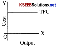
1. Total Fixed Cost (TFC):
It refers to the total money expenses incurred on all the fixed factors in the short run. TFC remains constant at all levels of output. Therefore the total fixed cost curve is horizontal straight line parallel to x axis above the origin which indicates that it is never zero.

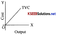
2. Total Variable Cost (TVC):
It refers to the total money expenses incurred on the variable factor inputs in the short-run. Total variable cost is the direct cost of the output because it increases along with the output and remains zero when the output is zero. So, the TVC curves starts from the origin and rises sharply in the beginning, gradually in the middle and stretches again sharply in the end. The nature of this slope is in accordance with the law of variable proportion.

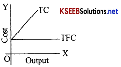
3. Total Cost (TC):
It is the aggregate money expenditure incurred by the firm on all the factors to produce a given quantity of output. TC varies in the same proportion as total variable cost because the total fixed cost is constant. The TC curve slope upwards from left to right, above the origin, indicating that, it includes total fixed cost and total variable cost.
TC = TFC + TVC

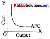
4. Average Fixed Cost (AFC):
It is the fixed cost per unit of output. In other words, it is average expenses incurred on a single unit of output produced. AFC and output are inverse relation i.e. AFC will be higher when the output level is less and as the output goes on increasing, AFC starts reducing. When it is represented in the diagram, AFC curve will have a negative slope which falls very stiffly in the beginning and later on becomes parallel to the X axis. This shows that it is never zero as TFC is never zero.
The Average Fixed Cost is obtained by dividing Total Fixed Cost by the output. AFC = TFC/output.

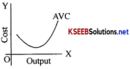
5. Average Variable Cost (AVC):
It is a variable cost per unit of output. It can be calculated by dividing total variable cost by the total units of output. When this cost is graphically represented, we get a ‘U’ shaped AVC, which shows that the cost will be less as the number of units produced.increase, this is because as the number of variable inputs are added in a fixed plant the efficiency will increase and vice versa.
AVC = TVC/output or AVC = AC – AFC

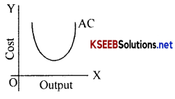
6. Average Cost (AC):
It is the cost per unit of output produced. It is obtained by dividing total cost by the total output produced i.e. AC = TC/Q or it is also obtained by adding AFC and AVC. If the AC is graphically represented, we get a U shaped curve because of the operation of law of variable proportions. The short run AC curve is also called as ‘Plant Curves’ because it indicates the optimum utilization of a given plant (Industry) capacity.

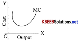
7. Marginal Cost (MC):
It is an additional cost incurred to produce an additional output. In other words it is the net additions to the total cost when one more unit of output is produced.
MC = TC_n – TC_{n – 1}
(Where TC_n = Total Cost of ‘n‘ selected units of output and TC_{n – 1} is total cost of the previous output)

Other types of costs:

1. Money Cost and Real Cost:
Private cost: Private costs, also referred to as Money costs, include all those expenses of’ producer expressed in terms of money. Example: Costs on rent, power, raw material, transport, expenses etc.

Real Cost: When cost is expressed in terms of physical or mental efforts put in by a person in the making of a commodity, it is called as real cost. It includes efforts, services and sacrifices put in by different factors of production. The concept of Real Cost was introduced by Prof. Alfred Marshall.

2. Explicit Cost and Implicit Cost:
Explicit cost is the external costs incurred by the producer on all those factors which is either hired or purchased by him.

Implicit cost: Implicit costs are imputed cost which is incurred on all those factors which are owned by t he producer himself. These costs are only book cost which is only accounted and not actually incurred. For example the salary of the owner, the depreciation charges etc.

3. Opportunity Costs:
The concept of opportunity cost was popularized by an American writer -Prof.Heberlour. It is the cost measured in terms of revenue earned by the factor when it is employed in some other alternative jobs. In other words it is the cost of displaced alternative. While calculating opportunity cost the profit earned from the best alternative employment sacrificed is taken into consideration. Therefore, opportunity cost is also called as Alternative Cost. If the factor decision doesn’t involve any sacrifice then its opportunity cost is zero.

4. Social cost:
The Social Costs are those expenses of the Government or Private Sector to produce goods and services for the entire society or economy. For example, to combat pollution, deforestation, flood etc, Government and NGO spend huge amount of money. This may be termed as Social Cost.

2nd PUC Economics Notes