Category: 2nd PUC

Karnataka 2nd PUC Statistics Notes Chapter 8 Operation Research

High Lights of the Topic:

→ Strategic problems relating to military forces, a group of scientists and experts, suggested appropriate allocations of available resources, and they helped in elficient handling the complex military operations, such as detection of enemy submarines, anti aircrafts, fire control etc, and they called the concept as Operations Research (OR).

→ However afterwards the science becomes popular, the applications (uses) of OR was applied to general problems such as, problems concerning Industry, Marketing, Personnel management, Inventory control, etc.

→ Therefore OR can be defined as “It is the method of application of scientific methods, techniques and tools to problems involving the operations of a system, so as to provide those in control of the system with optimum solutions to the problem.”

Scope:

Some of the problems in real life situations (problems) discussed in Operations Research (OR), are-
(i) Linear programming problems(LPP) are used in Industries for effective use of men, machine, money and material.

(ii) Transportation problem (TP) helps in shipment of quantities from various sources to different destinations at a minimum cost.

(iii) Game theory is applied in conflicting situations, to suggest the best strategy.

(iv) Replacement problems helps in suggesting the best time period to replace a specific part in manufacturing process, and

(v) Inventory problems help in organizing stocks and maintaining costs, and so on.

(i) Linear Programming Problem (LPP):

→ In many Economic activities, i.e. of Business and Industrial field, we often face the problems of decision making or optimization (may be Maximization/Minimization) of profit, sales, cost, labour etc, is very important. On the basis of available resources(called constraints), such as Demand for commodities, availability of raw materials, storage space, variation in costs, etc, In such situations where conditional optimization is required we may adopt ‘Linear programming’ model.

→ It was in 1947 that George Dantzig and his associates introduced the Linear programming technique and simplex method of solving problems concerning military activities.

→ Here “Linear programming is a mathematical technique which deals with the optimization (Maximization or Minimization) of activities subject to the available resources.”

For example:
1. A biscuit manufacturing factory may be interested in taking decisions regarding the type of biscuits to be manufactured and the quantity produced so as to earn maximum profit.

2. A factory having some machines to manufacture cars would like to know the best way to utilize the machines so that maximum production is made possible in minimum time available,

3. A dietician may want to suggest food with a certain basic vitamins and proteins. She may like to know the best way to prescribe food with optimum requirement of vitamins and proteins at the minimum cost.

Formulation of LPP:

• Identify the unknown variables- known as Decision variables and denote them in terms of algebraic symbols (as x,y).
• Identify the Objective of the problem and represent it as Z.
• Identify the restrictions called constraints in the problem and represent them as equations or inequalities in terms of symbols (as ≤ = ≥).

LPP Model :-
(Matrix Notation)                                      Optimize Z = CX
Subject to the constraints-                       AX(≤ = ≥)b
and the non-negativity restriction            X ≥ 0 ; is an LPP

Example:
A manufacturer produces two models of products Model A and Model B
(i) Model A fetches a profit of Rs.200/- per set. Whereas Model B fetches Rs.500/- per set.

(ii) Model A requires 6 units of raw material and Model B requires 3 units of raw material. Every week there is a supply of 180 units of raw materials.

(iii) Model A requires 4 hours and Model B requires 8 hours labour. The total labour available is 160 hours per week.

→ With the above facts, the manufacturer is to decide the number of Model A Products and number of Model B should he manufacture. In taking decision he should maximize his profit, on the basis of availability of Raw materials and the labour available.

→ The manufacturer’s problem can be mathematically written down (formulated) as follows:-

→ Let Y denote the number of units of Model A products to be manufactured. Let ‘y’ denote the number of Model B products to be manufactured. (x,y-decision variables)

→ Then, the manufacture’s profit is- (objective function)
Max. Z = 200x + 500y
(Restrictions are-) Subject to constraints; 6x + 3y ≤ 180
Since the weekly supply raw materials are 180 units, at the most 180 units can be utilized.
4x + 8y ≤ 160

→ Since total labour available is 160 hours.
Also the number of products cannot be negative, and so, X ≥ 0, Y ≥ 0
Thus, the formulated form of the the manufacturer problem (LPP) is;
Maximize = 200x + 500y
Subject to constraints, 6x + 3y ≤ 180.
4x + 8y ≤ 160
And non-negative restrictions: x,y ≥ 0 is an LPP

→ Definition: Linear programming deals with the optimization of a linear function of variables known as ‘objective function’ subject to a set of linear equalities / inequalities known as constraints.

→ Objective function: The function Z = CX which is to be optimized (Maximised/Minimised) is called Objective function. {E.g. Maximize = 200x + 500y}

→ Decision variable: A variables be ‘x₁, x₂, x₃ ………… x_n‘ whose values are to be determined are called decision variables.
{E.g: x, y variables}

→ Solution: A set of real values X = (x₁, x₂, x₃ ………… x_n) which satisfies the constraints AX(≤ = ≥)b is called a solution.

→ Feasible solution: A set of real values X = (x₁, x₂, x₃ ………… x_n) which satisfies the constraints AX(≤ = ≥)b and also satisfies the non-negativity restrictions x ≥ 0 is called feasible solution.

→ Optimal solutions:
A set of real values X = (x₁, x₂, x₃, ………. x_n) which

• Satisfies the constraints AX(≤ = ≥)b.
• Satisfies the non-negativity restriction x ≥ 0 and
• Optimizes the objective function Z = CX is called optimal solution

Note:

• If an LPP has one optimal solution, it is called to have unique optimal solution
• If an LPP has many optimal solutions, it is said to have multiple/Multiple Optimal solutions.
• For some LPP may not have optimal solution or the optimal value of Z may be infinity, in this case the LPP is said to be unbounded solution.
• In an LPP if all constraints cannot be satisfied simultaneously then there exists no solution to the given LPP.

Finding the solution to a LPP by graphical method:

• Consider the constraints as equality
• Find the co-ordinates for each constraint
• Draw the graph and represent by straight line
• Identify the feasible region-which satisfies the non-negativity restriction and constraints simultaneously
• Locate the corner points of the feasible region
• Find the value of the objective function at the corner points
• Get the optimum value and suggest the solution to the LPP

Note: Feasible can lie/exists only in First quadrant’: because for the given LPP, the solution . can exists only on xy-plane, because of the non-negativity restrictions, x and y both are positive on xy-plane.

(ii) Transportation Problem (T.P)

→ T.P was introduced by F.L.Hitchcock (in 1941) and T.C.Koopman (in 1947).

→ “The transportation problem (T.P) is a problem concerning transportation of goods from different origins (factories, warehouses/godowns) to various destinations (dealers, customers)”.

→ Here each origin has a certain stock of goods and each destination has a certain requirement of goods and there is a certain cost associated with transportation of goods from the various origins to the different destinations.

→ Following terminology are used of transportation problem:

• Let ‘m’ be the number of sources or origins.
• ‘n’ be the number of destinations.
• ‘ai’ be the quantity of goods available at i^th source
• ‘bj’ be the quantity of goods required at j^th destination.
• ‘Cij’ be the cost of transportation of unit of goods from i^th source to j^th destinations.
• And ‘xij’ be the number of units to be transported from i^th source to j^th destination.

→ Formulation of T.P:
Consider a T.P with ‘m’ origins O₁, 0₂ . . . . .O_m and ‘n’ destinations D₁, D₂ ….. D_n
Let ai be the quantity of product available at O_i
bj be the quantity of product required at D_j.
Cij be the cost of shipping of one unit of product from Oi to D_j
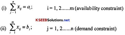
If xij is the number of units to be shipped from O_i to D_j. Then the problem is to determine xij so as to minimize the total transportation cost

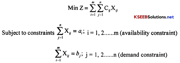
And, all x_ij ≥ 0 i = 1, 2 …………. m & j = 1, 2, ……. n.
Here, a T.P in which (availability) Σa_i = Σb_j (requirement) is called balanced TP

Definitions:
Feasible solution:
A set of values x_ij > 0, (i = 1, 2.. m and j = 1, 2 ….. n) is a feasible solution which satisfies:

→ Basic feasible solution(BFS): ‘A feasible solution is said to be a basic feasible solution if the number of non-zero allocations are (m + n – 1)’.
Here (m + n – 1) variables are known as basic variables.

→ Degenerate solution: When the number of positive allocations in any BFS is less than (m + n – 1), then the solution is said to be degenerate.

→ Non-degenerate solution: The number of positive allocations in any BFS is exactly (m + n – 1), then the solution is said . to be non-degenerate.

→ Optimal solution: A feasible solution is said to be optimal if it minimizes the total transportation cost.

→ Finding the initial solution:
An B.F.S. is obtained by :

• Northwest corner rule method (NWCR) ‘
• Matrix minima method(MMM)

→ Northwest corner rule method (NWCR):
In a given T.P. of m-origin, n-destination T.P. with ai-availabilities(i = 1, 2, 3 ……. m) and bj- requirements (j = 1, 2, 3 ……. n)an I.B.F.S is obtained as below:

Step I:
To start allocating at the cell (1, 1) which is north-west comer cell as: X₁₁ = min (a_i, b_j)

Step II:
(a) If a₁ > b₁ next allocation is made at the cell (1, 2) as: X₁₂ = min(a₁ – x₁₁, b₂)
{in the same row until the factory availabilities are allocated other dealers}

(b) If a₁ < b₁ next allocation is made at the cell (2, 1) as: X₁₂ = min(a₂, b₁ – x₁₁)
{in the same column where dealer’s requirement is satisfied from other factories}

(c) If a₁ = b₁ next allocation is made at the cell(2, 2)as: X₂₂ = min (a₂, b₂)
{where both dealer and factory are satisfied}

Step III:
The above procedure is repeated until all the availabilities of the origins are allocated to requirement of the different destinations.

Matrix minima method:
(Least/low cost entry method)
In a given T.P. of m-origin, n-destination T.P. with ai-availabilities(i = 1,2,3…m) and bj- requirements (j = 1, 2, 3 …….. n) an I.B.F.S is obtained as below:

Step I :
Identify the least cost in the cost matrix (called matrix minima) of the T.P. table.
Let C_ij be the least cost then allocation is made at the cell (i, j) as:
x_ij = min (a_i, b_j)

Step II:
(a) If a_i > b_j, jth column is deleted and ai is replaced by (a_i – x_ij ), repeat step I:
{here dealer is satisfied so deleted, factory availabilities are more}

(b) If a_i < b_j ith row is deleted and bi is replaced by (b_j – x_ij), repeat step I.
{here factory availabilities are exhausted}

(c) If a_i = b_j, ith row and jth column are deleted
{where both dealer and factory are satisfied}

Step III:
The above procedure is repeated until all the availabilities of the origins exhausted

(iii) Game Theory

→ Definition “Whenever there is a situation of conflict and competition between two or more opposing teams, we refer to the situation as a game” (It is science of conflicts)

→ In a game when each player chooses a possible action, then we say that a play of the game has resulted.

Assumptions/properties/characteristics of a competitive game

• There are finite numbers of players (competitors)
• Each player has finite number of course of action
• The game is said to be played when each of the players adopt one of the courses of action
• Every time the game is played the corresponding combination of courses of action leads to transaction (Payment) to each player. The payment is called pay off (gain).
• The gain of one player is exactly equal to the loss of the other

→ n- Person game:- A game in which n players participate is called n-person game.

→ Two-person game:- A game in which only two players participate is called two-person game.

→ Zero-sum game:- A game in which sum of the gains (pay-offs) of the players is zero is called ‘zero sum game’

→ Two-person-zero-sum game:- If in a game of two players, the sum of gain of one player is equal to the sum of loss of other is known as ‘two-person zero-sum game’. Also called as ‘Rectangular Game’.

→ Strategy:- In a game, the strategy of a player is the predetermined rule by which he chooses his courses of action while playing the game.

→ Pure strategy:- while playing a game, pure strategy of a player is his predetermined decision to adopt a specified course of action irrespective of the course of action of the opponent.

→ Mixed strategy:- While playing a game, mixed strategy of a player is his pre-decision to choose his course of action according to certain pre-assigned probabilities.

→ Optimal strategy:- A strategy of the game which maximizes the gain of one player and minimizes the loss of the other player is called optimal strategy.

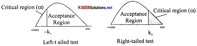
→ Maximin:- Maximum of the row minimums in the payoff matrix is called Maximin. max

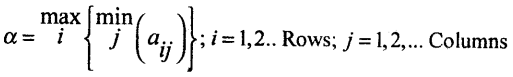
→ Minimax:- Minimum of the column maximums in the payoff matrix is called minimax.

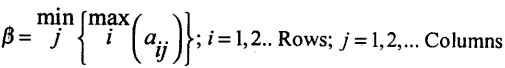
→ Saddle point:- Saddle point is the position where the maxmin and the minimax coincide – i.e. α = β = v

→ Value of the game:- Common value of maxmin and minimax denoted by ‘V’.

→ Fair game:- If the value of the game is zero, then the game is called fair game otherwise unfair.

I. Solution to a game with saddle point:-

The saddle point of the game is found as follows:
1. The minimum payoff in each row of the payoff matrix is circled as : ○

2. The maximum payoff in each column is boxed as: ▢
→ In the above process, if any payoff is circled as well as boxed, that payoff is the Value of the game (v).
The corresponding position is the saddle point

→ Indicate the position of the saddle point, and then suggest the strategy for players.
Also, write down the value of the game.

II. Principle of dominance:
→ When Two-person Zero-Sum game has no saddle point, the Maximin-Minimax principle breaks down. In such situation, we use other method called the principle of dominance to find the optimal strategy and value of the game.

→ “If the strategy of a player dominates over the other strategy in all conditions, then the latter strategy can be ignored because it cannot affect the solution in any way”

Rules:
1. If all the elements in a row (say i^th row) of a payoff matrix are greater than or equal to the corresponding elements of the other row (say j^th row) then i^th row dominates j^th row , then j^th row can be deleted.

2. If all the elements in a column (say r^th column) of a payoff matrix are less than or equal to the corresponding elements of the other column (say s^th), then r^th column dominates s^th column. So s^th column casn be deleted.

Repeat the process till optimal strategy is obtained.
Note:- To Get a Transpose of a matrix write a_ij to – a_ji Rows into columns with sign change.

(iv) Replacement Problems

Replacement theory deals with the problems of deciding the age at which the old equipments (machine and their spare parts, trucks etc.) are replaced.

Need: New equipments will generally be more efficient and their maintenance cost would be less. As they become old, their efficiency decreases and their maintenance cost (running, operating) increases. Also to determine optimum time for replacement of machine, trucks and equipments.

Following are the needs:

• As the equipment grows older, the maintenance would be costlier.
• New equipments would be more efficient than the old ones.
• Technology of new equipment would be superior to that of the old.
• Production/working cost would be lesser in new equipments.
• Modern equipments are more beautiful and more compact than old equipments.

Replacement of equipments, which deteriorates with age:
Machine and their spare parts, trucks etc. deteriorates with time, their maintenance cost increases and efficiency reduces. Hence, their replacement becomes necessary. Therefore, purchasing cost, resale value, maintenance cost etc. change with time. However, here we are not considering change in the money value.

The Average annual cost is- A(N) = \(\frac{\mathrm{T}}{n}\)
Where P = capital (purchasing) cost of an equipment;
S_n = Resale value (scrap value, salvage cost) of an equipment at age ‘n’
C_i = Maintenance cost at time i = 1, 2,…. n years
The optimal replacement time is that value ‘n’ for which A(n) is least. Ie the equipment is suggested to replace at that period Where the Annual Average Cost A(n) ceases to decrease,

(v) Inventory Problems

→ An Inventory is a physical stock of goods, which is held for purpose of future production or sales.

→ Inventory may be that of

• Raw materials
• Finished goods
• Semi finished goods.

→ A problem concerning such a stock of goods is Inventory problem. The object of analysis of inventory problem is to decide when and how much to be acquired, so that the cost is minimized and profit is maximized.

Need:
An inventory is essential for the following reasons:-

• It helps in smooth and efficient running of the business.
• It provides adequate and satisfactory service to the customers.
• It facilitates bulk purchase of raw materials at discounted rates.
• It acts as buffer stock in case of shortage of raw materials.
• Inventory is also needed to optimize the cost.

However, the inventory has disadvantages such as, warehouse rent, labour of maintenance loss due to fall in price, interest on capital invested, deterioration of goods etc.

Variables in the inventory problem:
The variables involved in the inventory are of two types:

1. Controlled variables .
2. Uncontrolled variables

1. Controlled variables:
1. The variables, which can be controlled individually or jointly, are called Controlled variables. They are

• Quantity of goods acquired.
• Frequency or timing of acquisition or replenishment.
• The completion time or stage of stocked items/production of stocked items.

2. Uncontrolled variables: The variables, which cannot be completely controlled are called Uncontrolled variables. These include “Purchase/Capital cost, Carrying cost (Holding / Storage / Maintenance cost), Shortage/Penalty cost and Set-up cost (Replenishment / Ordering cost)”.

Note: Total inventory cost =Purchasing cost (P) + Setup cost (C₃) + Holding cost (C₁) + Shortage cost (C₂)
Inventory costs These are inventory costs associated with keeping inventories. They are

(a) Purchasing cost (P): It refers to the cost associated with an item whether it is manufactured or purchased. (Also called as Capital cost)

(b) Set up cost (C₃): It is the cost of setting up the machines for production or the cost of placing the order for the goods: It includes labour cost, transportation cost etc. It is also called as ordering cost, Replenishment cost, or Procurement cost. Denoted by C₃.

(c) Holding cost (C₁): It is the cost associated with carrying or holding/ the goods (Inventory) in stock until the goods are sold or used. (It includes rent for space, interest on capital invested, maintenance of records, taxes, insurance and breakages.)
Here Carrying cost (C₁) is also the percentages (%) of the capital cost. So C₁ = PI
Holding/Carrying cost per unit time per unit good is denoted C.

(d) Shortage cost (C₂): The cost associated with delay or inability to meet the demand because of shortage of stock is called shortage cost. Also called as penalty cost-C₂.

→ Demand (R):- Demand is the number of units required from the inventory per period. If the demand remains fixed, is called deterministic demand. If the demand varies randomly, is called probabilistic demand

→ Lead time: – The time gap between placing of order and arrival of goods at the inventory is the Lead time (Delivery lag)

→ Stock replenishment:- The rate at which items are added to the inventory to maintain a certain level is known as stock replenishment.

• The quantity of goods acquired in one replenishment is the Order quantity (Q) {Lot size, Run size, Stock replenished}
• The number of times replenishment is done in unit time (year) is the Frequency of replenishment
• The time gap between two replenishments is the Re-order time (t) {Re-scheduling time, production run}

→ Quantity delivered (Depletion): It is the number of units of goods delivered.

→ Time horizon (T): The period over which inventory level is maintained is called Time horizon.

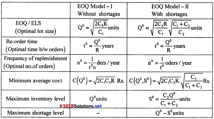
→ The Economic Order Quantity (EOQ): The EOQ is the size of the order for which the aggregate of setup cost and holding cost of the Inventory is minimum.

(a) EOQ/ELS model with

• Uniform demand
• Instantaneous production/supply
• Shortages not allowed.

→ Inventory problems where demand is assumed to be fixed and pre-determined are called EOQ/ELS

→ A set of mathematical equations required to solve an Inventory problem is called an Inventory Model.

→ Inventory Model, which are meant for deterministic demand are called EOQ Model or Economic Lot Size (ELS) model.

The Assumptions for this Model are:

• Demand is deterministic and uniform
• Production or stock replenishment is instantaneous
• Shortages are not allowed
• Lead Time is zero
• Setup cost is Rs.C₃ per cycle (production run)
• Holding cost is C₁ per item per year
• Time period for maintaining of the level of Inventory is 1 year

Notations:

• Q – Lot size (run size, Quantity replenished, order quantity)
• P – Purchase/Capital cost,
• R – Demand Rate,
• S – Initial Level of Inventory,
• t – Time interval between two consecutive replenishment (Rescheduling time)
• n – Number of replenishment per unit time
• C₁ – Carrying (Holding cost, Storage cost, Maintenance cost) per unit good per unit time
• C₂ – Shortage cost/Penalty cost per unit good per unit time
• C₃ – Setup/ordering cost per production run
• I – Carrying/Holding Cost per Rupee per unit time,
• C (Q) or C(Q°, S°) – Average cost per unit time.

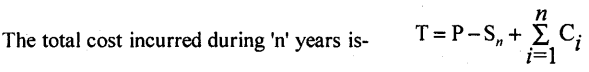
Diagram of EOQ Model-I without shortages

Here the initial level Q of the inventory depletes in time t at the rate R to the zero level. After time t, then Inventory is replenished by Q units and the cycle continuous. Here ?OAB indicates the Inventory carried.

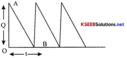
Diagram of EOQ Model-II with shortages

Here at the time of replenishment, there would be a shortages (Q-S) units and so, the level of inventory would be S. This level depletes in time t₁ to zero. Here ?OAB represents the Inventory carried and ∆BCD represents the shortage carried.

2nd PUC Statistics Notes

Karnataka 2nd PUC Statistics Notes Chapter 7 Statistical Quality Control

High Lights of the Topic :

The Quality control and Statistical quality control (SQC):
→ “statistical quality control is the method of controlling the quality of the products using statistical techniques”.

→ Here the term ‘quality’ refers to a characteristic of a product which satisfies the standards specified for measurement.

Sources of Variation:

The variation in quality of goods may be due to

1. Chance causes and
2. Assignable causes.

1. Variation due to chance causes:
→ These are called common or random causes of variation. These types of variation are unavoidable and are due to slight differences in processing.

→ ‘A small amount of variation for which no specific cause can be attributed (recognized) is termed as chance causes of variation’.

→ Chance variation causes cannot be reduced or eliminated by any statistical means. Hence one has to tolerate such variations and this variation is called natural tolerance.

2. Variation due to assignable causes:
→ The second type of ‘variation that can be observed in the quality of the product and the causes can be identified and eliminated. These are called assignable causes of variation’.

→ Causes of these type of variation may be due to-use of substandard quality of raw material, un even supply of electrical voltage, untrained men handling the machine, improper functioning of machine etc., These causes of variation can be identified and eliminated.

→ The manufacturing process has following stages. They are

1. Specification/product specification
2. Production
3. Inspection

1. Specification/product specification: Specification is the quality standards of measurements fixed for an item to be produced. An item produced from the production process according specifications, is called production. Verification of the quality standards of the manufactured item is inspection.

Uses / Need / Advantages of SQC:
SQC is very essential because

• To improve the quality of items and to decrease the proportion of defectives.
• To eliminates faults and prevents the loss due to spoilage and rework by timely identification of assignable causes.
• To prevent the financial loss- by changing the production method if the production process goes out of control.
• Manufacturer can guarantee or warranty his product with confidence.
• It provides greater quality assurance at lower inspection cost. ,
• The very presence of SQC department, alerts the workers in the production plant.
• The quality control technique has two different stages in production process:

(i) Process control:
‘Controlling the quality of the goods, during the manufacturing process itself is called process control’. That is, a production process is said to be in statistical control if the products are free of variations due to assignable causes.

(ii) Product control:
‘The process of inspection of manufactured lot for acceptability is called product control or acceptance sampling’.

Variables and Attributes:-
→ If the record of the actual measurements of quality characteristics for an individual item are specified, we use averages and standard deviations.

→ ‘A measurable quality characteristic which varies from unit to unit is Variable’.
ie., generally expressed with statistical measures such as averages and standard deviations (range). Where sophisticated instruments (caliper) used to measure.

Example 1:
→ Length, Breadth, Ht, Wt, Resistance, thickness, tensile strength of articles, volume, of the manufactured articles, Other examples are the weight of a bag of sugar, the temperature of a micro oven, or the diameter of plastic pipes, etc.,

→ X̄ and R charts are used for the control of variables.

→ ‘A qualitative characteristic which cannot be measured and can only be identified by its presence or absence is an Attribute’.
ie., a performance characteristic that is either present or absent in the product or service under consideration. Most quality characteristics in service industry are attributes

Example 2:
→ Broken, cracks, scratches, bubble, improper less/more colour painting/tint of articles/glass dome number of broken Potato chips, infested apples, improper reflection of mirror, spots of uneven thickness or folds in paper, knitting defects on a cloth etc.,

→ np-charts and c-charts are used for control of attributes.

Defects and Defectives:

→ ‘A defect is a quality characteristic which does not conform to specifications.’

→ Misprints, damages in weaving of a cloth, a bubble in the glass bottle, excessive thickness of a glass pane, an infest in apple, a fold or scratches in paper and example 2 are all defects.

→ ‘An item having one or more defects is a defective item’.

→ The cloth with misprints, glass bottle having air bubbles, excessive thickness of a glass pane are all defectives.

3σ – limits:

→ We know that mean-X̄ and S.D-σ follows a normal variate and so, assuming that the production process follows a normal distribution/curved then, from the area property of Normal distribution: P(µ – 3σ < X < µ + 3σ) = 0.9974.

→ “In the constructing control charts, control limits are nothing but 3 o-limits. If the manufacturing process is said to be in control, then 99.73% of observations lies within 3 o-limits”. Here almost all chance causes are within control limits, if not, is an indicator of presence of Assignable causes.

Developing Control Charts:

→ A control chart is a graph that shows whether a sample of data falls within the common or normal range of variation.

→ “Control chart is a graphical device which is used to verify whether the production process is under statistical control or not”.

→ A control chart has upper and lower control limits that separate common from assignable causes of variation. A control chart consists f three horizontal lines.

Quality Standards for control limits:

→ For drawing the control charts we need parameters (standards). If the parameters are available from past production process/ experience/expected and if they are well accepted we say that they are known standards.

→ If the standards known are denoted by X̄’ – mean, S.D – σ (for X̄, R-charts), P¹ – fraction/ proportion of defectives (for np-chart) and λ’ – average defects (for c-charts).

→ If a control chart is being constructed for a new process, the mean (µ) and σ (the population parameters) will not be known and hence must be estimated from the sample data, then we say that standards are not known.

→ If the standards not known are denoted by X̄, R̄ (for X̄ > R-charts), p̄ (for np-chart) and c̄ (for c-charts).

Control Charts for Variables:

For mean/averages and s.d/ranges-

Where X̄’, σ’ are given standards, and if not given, X̄ = \(\frac{\sum \mathrm{x}}{\mathrm{n}}\) and X̿ = \(\frac{\sum \mathrm{x}}{\mathrm{k}}\) also R̄ = \(\frac{\sum \mathrm{R}}{\mathrm{k}}\) where K is the number of samples/sample no./subgroup no. The constants A, A₂, d₂, D₁, D₂, D₃ and D₄ are referred from the tables for for samples n = 4/5. {only for X̄ and R-charts}

Control Charts for Attributes:

Suppose samples of size ‘n’ are drawn at regular intervals and ‘d’ is the no. of defectives in each of these samples. Then ‘d’ is a Binomial variable with mean ‘np’ and standard deviation √nPQ, where P is the probability that an article is defective.

The control limits for the np/d-(defectives) chart:

→ Where P’ is the proportion of defective the given standard and Q’ = 1 – P’, if not given: p̄ = \(\frac{\Sigma \mathrm{d}}{\mathrm{nk}}\);

→ where n-sample size and p̄ = \(\frac{\text { Total number of defective items }}{\text { Total number of observations in k samples }}\)

C – Chart for number of defects: Suppose ‘c’ denotes the number of defects per unit. Then ‘c’ is a Poisson variable with mean λ and standard deviation √λ, where λ is the average number of defects per unit in the population. The control limits for c – charts are as follows:-

The control limits for c – charts:

Where c̅ = \(\frac{\Sigma \mathrm{c}}{\mathrm{K}}\) is average number of defects.

Interpretation of control charts (Detection of Lack of control):
We say that a process is out of control when a plot of data reveals that one or more samples fall outside the control limits.

• One or more points lie outside the control limits.
• A run of seven or more subsequent points lie to one side of the central line.
• Upward or downward trend in the points.
• Presence of cyclical variation in the points.

Acceptance sampling plan:
→ “The process of inspection manufactured lot for acceptability is called acceptance sampling plan”.
Manufactured lot can be verified either by

• 100% inspection ie. by verification of each and every item of the manufactured lot or
• Sampling techniques: A sampling plan is a plan for acceptance sampling that precisely specifies the parameters of the sampling process and the acceptance/rejection criteria.

→ In acceptance sampling there are two methods(sampling plans). They are

1. Single sampling plan and
2. Double sampling plan.

Merits:

• It helps to decide whether or not desirable quality has been achieved for a batch of products.
• It is used when the items are of destructive in nature.
• It is less expensive.

Demerits:

• There is a risk of accepting a bad lot and rejecting a good lot.
• Costly and time consuming.

1. Single sampling plan (SSP):
→ In SSP where a random sample of items are drawn from every lot. Each item in the sample is examined and is labeled as either good or bad, depending on the number of defects or bad items found, the entire lot is either accepted or rejected.

→ “In a single sampling plan, the decision about accepting or rejecting a lot is based on one sample only.”

→ In this method, in a lot of size N, the sample size ‘n’ is drawn from the lot and’d’ be the number defectives in the sample and ‘c’ be the maximum number of defects at which a lot is . accepted. These parameters define the acceptance sampling plan.

Then SSP is :

• If d ≤ c, accept the lot and replace ‘d’ defectives by good ones.
• If d > c, the entire lot is inspected and all defectives are replaced.

2. Double sampling plan(DSP):
→ This provides an opportunity to sample a lot a second time if the results of the first sample are inconclusive.

→ “In a double sampling plan, the decision is based on two samples drawn from a lot.”

→ Let N be the lot size, let n, and n2 be sample sizes of first and second samples. Let c₁ and c₂ be two acceptance numbers (here c₁ < c₂).

Then DSP is:-

• If d₁ ≤ c₁ accept the lot, where d₁ – no of defectives in the n₁ samples
• If d₁ > c₂, reject the lot. Inspect the entire lot and replace the didefectives by good ones.
• If c₁ < d₁ ≤ c₂, another sample n₂ is drawn from the lot.
• If (d₁ + d₂) ≤ c₂ accept the lot. Where d₂ – no. of defectives from second sample, However (d₁ + d₂) defectives are replaced by good one.
• If d₁ + d₂ > c₂ Reject the lot, inspect the entire lot and replace all defectives by good ones.

Merits and Demerits:

→ S.S.P is easier and simpler than the D.S.P.

→ Manufacturer feel more assured psychologically (regarding the defectives) in D.S.P than S.S.P.

→ In D.S.P in case the lot is accepted at the first stage itself, there would be reduction in the number of items inspected. And so, on an average the inspection cost would be less in D.S.P. than SSP.

2nd PUC Statistics Notes

Karnataka 2nd PUC Statistics Notes Chapter 6 Statistical Inference

High Lights of the Topic:

Parameter:

→ A statistical constant of the population is called a parameter.

→ Statistical constants of the population such as Mean (x̄), S.D (σ) & Proportion-P₀ Or P are Parameters

Parameter space:
→ The set of all the admissible values of the population parameter is called parameter space. Suppose X ~ N(µ, σ²), then parameter space for µ = {- ∞ < µ < ∞} and for a = σ = {0 < σ < ∞}

Statistic:
→ A function of the sample values is called a statistic.

→ Statistical measures computed from the samples such as Mean (x), S .D (s), & proportion- p are statistic.

Sample space:

→ The set of all samples of size W that can be drawn from population is called sample space.

Sampling distribution:

→ The distribution of the values a statistic for different samples of same size is called its sampling distribution.

→ Many sample means (x) can be tabulated in the form of frequency distribution from the population, the resulting distribution is called sampling distribution of sample mean (X̄). Similarly sampling distribution of sample S.D (s), sampling distribution of sample proportion (p) etc.

Standard Error:

→ The standard deviation of the sampling distribution of sample statistic is called standard error (S.E) of statistic

S.E (X̄) of sample mean:

Consider a population whose mean ‘μ’ and S.D. ‘σ’. Let a random sample of size ‘n’ be drawn from this population. Then the sampling distribution of X̄ has mean ‘μ’ and Standard deviation:
SE(X̄) = \(\frac{\sigma}{\sqrt{n}}\)
If ‘σ’ is not available use’s’, SE(X̄) = \(\frac{\mathrm{s}}{\sqrt{\mathrm{n}}}\) =; s-sample S.D

S.E of difference of means/ S.E(x̄₁ – x̄₂):
→ Let a random sample of size ‘nl’ be drawn from a population whose mean is µ₁, and s.d. σ₁. Also, let a random sample of size ‘n₂‘ drawn from another population whose mean is µ₂, and s.d. σ₂. Let x̄₁ and x̄₂ are the means 1st and 2nd samples drawn from the populations,

→ Then difference of sample means (x̄₁ – x̄₂) has mean ‘(µ₁ – µ₂)’ and
S.E. (x̄₁ – x̄₂) = \(\sqrt{\frac{\sigma_{1}^{2}}{n_{1}}+\frac{\sigma_{2}^{2}}{n_{2}}}\) OR S.E. (x̄₁ – x̄₂) = \(\sqrt{\frac{s_{1}^{2}}{n_{1}}+\frac{s_{2}^{2}}{n_{2}}}\); Where s₁ and s₂ are sample standard deviations

S.E of sample proportion/ S.E (p₁ – p₂):
→ In a population let PQ be the proportion of units which posses the attribute. From such a population suppose a random sample of size ‘n’ is drawn.

→ Let ‘x’ of these units belongs to the class ‘posses the attribute’ then p = \(\frac{x}{n}\), is the sample proportion of the attribute. Then ‘p’ has mean ‘P0’ and S.E(p) = \(\sqrt{\frac{\mathrm{P}_{0} \mathrm{Q}_{0}}{\mathrm{n}}}\); Q₀ = 1 – P₀

→ Here, in order to avoid confusion between population proportion (P) and sample proportion (p): ‘caps’ P is used as P₀ and Q as Q₀

S.E. of difference of the sample proportions/S.E (p₁ – p₂):
→ Let a random sample of size ‘n₁‘ be drawn from a population with proportion ‘P₀₁‘ of an attribute. Let x₁ units in the sample posses the attribute. Then the sample proportion of 1 st sample: P₁ = \(\frac{x_{1}}{n_{1}}\).

→ Similarly n₂ → P₀₂; x₂ → p₂ = \(\frac{\mathrm{x}_{2}}{\mathrm{n}_{2}}\).

→ Hence the difference of (p₁ – p₂) has mean (P₀₁ – P₀₂) and S.E(p₁ – p₂) = \(\sqrt{\frac{\mathrm{P}_{01} \mathrm{Q}_{01}}{\mathrm{n}_{1}}+\frac{\mathrm{P}_{02} \mathrm{Q}_{02}}{\mathrm{n}_{2}}}\)

→ If P₀₁ = P₀₂ = P₀, ie, two population proportions are same, the
S.E (p₁ – p₂) = \(\sqrt{\mathrm{P}_{0} \mathrm{Q}_{0}\left(\frac{1}{\mathrm{n}_{1}}+\frac{1}{\mathrm{n}_{2}}\right)}\)

Uses (utility) of S.E’s :

• It is used in theory of estimation, to decide the efficiency and consistency of the statistic as an estimator.
• It is used in interval estimation, to write down the confidence intervals.
• It is used in testing of hypothesis, to test whether the difference between the sample statistic and the population parameter is significant or not, ie. to standardize the distribution of test statistic.

Theory of Estimation:
→ The statistic used for the purpose of estimation of unknown population parameter is called an Estimator. Whereas Estimate is a numerical value of the computed from a given set of sample values.

→ Suppose if a sample statistics (x̄) is used to find out the value of the population parameter (µ), such a value is called the Estimator of the parameter. And the value of the Estimator is called the Estimate.

→ Thus, the statistic x̄ is an Estimator of µ and its value x̄ is the Estimate.

→ Similarly ‘s’ (sample s.d) is an Estimator of ‘σ’ (population s.d) and its value ‘s’ is the Estimate.

→ When estimating parameters of the populations, the following two types of estimates are possible.

1. Point Estimation
2. Interval Estimation.

1. Point Estimation:
In Point Estimation a single statistic used to provide an estimate of the population Parameter. “While estimating unknown parameter, if a single value is proposed as an estimate is called point estimation”
{i.e., the estimate of a population parameter given by a single number is called point estimation.} for example the mean pass number of 50 students will be 55.

2. Interval Estimation:

→ If an interval is proposed as an estimate of the unknown parameter, then it is interval estimation.

In Interval Estimation:

• “While estimating an unknown parameter, instead of a specific value, an interval is proposed, which is likely containing the parameter is called Interval estimation”
• A confidence interval is an interval within which the unknown population parameter is expected to lie. (The interval which is likely to contain the parameter)
• The probability that the confidence interval contains the parameter is called confidence coefficient.
• The Intervals within which the most probable value of parameter contains are called confidence limits. Ie the limits T₁ and T₂ of the confidence interval are called confidence limits.

Testing of Hypothesis

Statistical Hypothesis:
A statistical Hypothesis is a statement regarding the statistical distribution of the population OR It is a statement/assertion made regarding the parameters of the population denoted by H.
Ex:- H: The population has mean = p (= 25)
H: The population is Normally distributed with mean µ = 25, and s.d. σ = 2

Null Hypothesis:
“Null Hypothesis is a hypothesis which is being tested for possible rejection under the assumption that it is true. Denoted by H₀”
Ex: H₀: The population mean is µ (= 25) OR {H: µ = µ₀}
H₀: The means of the two populations are equal OR {H₀: µ₁ = µ₂}

Alternative Hypothesis:
“The hypothesis which is being accepted when the null hypothesis is rejected is called alternative hypothesis. Denoted by H₁”
Ex: H₁: The population mean differs from (H₁: µ ≠ µ₀ (25))
Also H₁ may be H₁: µ < µ₀(25) or H₁: µ > µ₀(25)
H₁: The means of the two populations are not equal, may be less than or more than
{H₁: µ₁ ≠ µ₂ or H: µ < µ₂ or H₁ = µ₁ > µ₂}

Simple Hypothesis:
“A hypothesis which completely specifies the parameter of the distribution is called simple hypothesis”.
Ex: H: < µ₀ (25) is a simple hypothesis
H: The population is Normally distributed with mean µ = 25 and σ = 2

Composite Hypothesis:
“A hypothesis which does not completely specify the parameter of the distribution is a composite hypothesis”
Ex: H: The population is normally distributed with mean µ > 25

Test statistic:
→ “Test statistic is the statistic based on whose distribution testing is conducted”

→ Suppose for testing H₀ = µ = µ₀, the test statistic is Z = \(\frac{\overline{\mathrm{x}}-\mu}{\mathrm{S} . \mathrm{E}(\overline{\mathrm{x}})}\) i.e., Z = \(\frac{\overline{\mathrm{x}}-\mu}{\sigma / \sqrt{\mathrm{n}}}\) OR Z = \(\frac{\overline{\mathrm{x}}-\mu}{\mathrm{s} / \sqrt{\mathrm{n}}}\)

→ Here “the statistical distribution of the test statistic under which the Null Hypothesis stated is called Null Distribution”

Critical Region:
→ “The set of all those values of the test statistic which lead to the rejection of the null hypothesis is called critical region (to), also called as Rejection region”.

→ “The set of those values of test statistics which lead to the acceptance of the null hypothesis is called acceptance region(s – ω)”.

Critical value:
→ “The value of test statistic which separates the critical region (i.e. rejection region) and acceptance regions is called the critical value or significance value”.

→ Usually denoted by ± K/-K₁, K₂. Its value depends of level of significance (α) used ie, either at 5% (0.05) or 1% (0.01).

Here for α = 5% ± K₁ = ± 1.96 and ± k₂ = ± 2.58 for two tail test
for α =1 % ± K₁ = ± 1.65 and ± k₂ = ± 2.33 for one tail test

When a statistical hypothesis is tested there are four possible decisions are made as below:

1. If the Null hypothesis is true and our test accepts it -Correct decision
2. If the Null hypothesis is true but our test rejects it -Type I Error
3. If the Null hypothesis is false and our test accepts it -Correct decision
4. If the Null hypothesis is false but our test accepts it – Type II Error

Type I:-
“Type I Error is taking a wrong decision to reject the null hypothesis when it is actually true” ie. (Rejecting H₀ when it is true)

Type II Errors:-
“Type II Error is taking a wrong decision to accept the null hypothesis when it is actually not true” (Accepting H₀ when it is not true)

Level of Significance (α):
“It is the probability of rejecting the null hypothesis when it is actually true denoted by α”.
i. e., α = P (Type I Error) OR ‘prob. of occurrence of Type I error is called Level or significance’, which is referred as ‘producers risk’. Usually is fixed at 0.05 or 0.01.
Here α = P (Type I Error) is also called as Size of the test.

Power of a Test:
“It is the probability of rejecting the null hypothesis when it is not true, denoted by (1 – β)”. ie., Here β = P(Type II Error) which is referred as ‘consumers risk’

One-Tailed and Two-Tailed Test:
→ While testing of null hypothesis, a two-tailed test of hypothesis will reject the H₀ if the sample statistic is significantly higher than or lower than the parameter.

→ Thus in two-tailed test the rejection region is located in both the tails.

→ Whereas is one tailed test rejection region is located in one side ie. Right or left tailed.

Definition:
→ “If the critical region is considered at one tail of the null distribution of the test statistic, the test is one-tailed test”
Ex:- When H_o: µ = µ₀ versus H₁: > µ₀, then it is a right tailed test;
When H_o: µ = µ₀ versus H₁: < µ₀, then it is a left tailed test.

Definition:
“If the critical region is considered at the both the tails of the null distribution of the test statistic, the test is two-tailed”

Ex:- When H₀: µ = µ₀ versus H₁: µ ≠ µ₀, then it is two tailed test.
When H₀: µ₁ = µ₀ versus H₁: µ₁ ≠ µ₀, then it is two tailed test.

Test Procedure:
Following are steps involved in any test of hypothesis:

• Setting up null and alternative hypothesis, ie., H₀ & H₁
• Identifying the test statistics and its distribution as, Z, χ², t, etc.,
• Selecting level of significance (α) and finding the critical value.
• Making decision and conclusion.

2nd PUC Statistics Notes

Karnataka 2nd PUC Statistics Notes Chapter 5 Theoretical Distribution

High Lights of the Topic:

→ The probability distribution of a random variable obtained on the basis of some theoretical assumptions are known as theoretical or probability distributions.

→ Discrete probability distributions: Probability distribution of a discrete random variable is known as discrete probability distribution.

Ex: Number of Heads obtained when three coins are tossed, Number of female children in a family, Number of accidents occurring in a city in a day, drawing balls without replacement from a bag of different coloured balls etc. are discrete variable examples. The following probability distributions are used to deal such examples.

• Bernoulli distribution
• Binomial distribution
• Poisson distribution
• Hyper-geometric distribution

Continuous Probability Distributions:
Probability distribution of a continuous random Variable is known as continuous probability distribution.

Ex: Height/ Weight/ Marks obtained by a of class of students, Age/Wages/Income of employees of a factory etc. are all continuous variable examples. The following probability distributions are used to deal with such examples.

• Normal distribution
• Chi-square distribution
• Student’s t-distribution

Discrete Probability Distributions:

Bernoulli Distribution:

{Introduced both Bernoulli and Binomial distributions by Mr.James Bernoulli} A random experiment which has only two outcomes as ‘success’ and ‘failure’ where
P(succeess) = p & P(failure) = q or (1 – p) is called Bernoulli Trail or Experiment.

Examples:
1. Tossing a fair coin once, and getting out comes as Head (success-p) or Tail (failure-q)

2. A new born baby may be male (p) or female (q)

3. A bomb is dropped on a target may hit (p) or may not hit (q)

4. An item chosen at random may be defective or not

5. Rolling a die and getting no. 6 (success) or not (other numbers). The probability mass function (p.m.f) is:
P(x) = P^x (1 – P)^{1 – X};                             where p > 0, and X = 0, 1
OR P(x) = P^x q^{1 – x} x = 0, 1                   Where p is probability of success (0 < p < 1)

→ Here x-is discrete and is called Bernoulli variate.

• The Bernoulli distribution with the parameter p denoted by B(p)
• The distribution can also be written as:

→ A random variable x assumes values 1 and 0 with respective probabilities p and (1 – p) is called Bernoulli variate
The Bernoulli distribution can also be writtens is:

Where p-the probability of success

Properties/Features:

• Here p-is the parameter, is a constant
• Mean = E(x) = p,
• var(x) = p (1 – p) or pq
• For the distribution Mean(p) > Variance
  s.d(x) = \(\sqrt{p(1-p)}\) or \(\sqrt{p q}\)

Binomial Distribution:

Bernoulli distribution tends to Binomial distribution:
If x₁, x₂, x₃ …………. x_n are independently identically distributed (i.i.d.) Bernoulli variates, then (x₁ + x₂ + x₃ + ………… + x_n) is a Binomial variate with parameters n and p

Conditions/Assumptions that Binomial distribution can be applied:

• Trails are repeated number of times and are independent.
• Each trail is a Bernoulli trial with two outcomes as success and failure
• The probability of success ‘p’ should be constant for each of the trails
• Experiment should be conducted under similar conditions for a fixed number of trails say ‘n’.

Examples:

• Number of heads obtained when 5 coins are tossed
• Number of male children in a family of 3 children
• Number-of defective articles in a random sample of 7 articles
• Number of bombs hitting a target when 4 bombs are dropped on it.

Similarly number of accidents, deaths, infections, contracting a disease, literates, mango trees among the trees etc.
The p.m.f is: P(x) = nc_xP^xq^{n – x}; Where x = 0, 1, 2, 3 …………….. n, and range of p: 0 < P < 1
Here x is discrete and is called Binomial variate.

Properties / Features:-
→ n & p are the parameters

→ Range: 0, 1, 2, n

→ The Binomial distribution with the parameters n, p denoted by B(n, p)

→ Mean = np, var(x) = npq, sd(x) = √var(x) = \(\sqrt{\mathrm{npq}}\)

→ Relation between mean and variance: mean > variance, ie. np > npq

→ Binomial distribution is symmetric when p = \(\frac{1}{2}\) (i.e., β₁ = 0 non-skewed).

→ Expected /Theoretical frequency = T_x = p(x).N

→ The distribution is called symmetric when p = q

→ Recurrence relation to get theoretical frequency = T_x = \(\frac{n+1-x}{x} \frac{p}{q} T_{x-1}\)

→ Recurrence relation to get theoretical P(x) = \(\frac{n+1-x}{x} \cdot \frac{p}{q} p_{x-1}\)

→ The terms of B.D are:

→ If p > \(\frac{1}{2}\) or q >\(\frac{1}{2}\) then binomial distribution is positively skewed (i.e., β₁ > 0).

→ If P < \(\frac{1}{2}\) or q < \(\frac{1}{2}\), then binomial distribution is negatively skewed (i.e., β₁ < 0).

Poisson Distribution

{French mathematician S.D.Poisson ini 837 used to describe the behavior of rare happening of events.}

Examples:

• Number of telephone calls received in one minute
• No. of printing mistakes in a book/typing mistakes (typographical errors) in a page.
• No. of accidents/deaths occurring in a city in a day
• No. of defective articles manufactured in a lot by a firm.
• Number of vehicles crossing a junction in one minute.

Binomial distribution tends to Poisson distribution under the following conditions:
(i) When n is large ie., n → ∞
(ii) When P is very small ie., p → 0 and
(iii) Mean = np = λ is fixed / constant, which is parameter of the Poisson distribution Poisson distribution is:
A distribution which has the following p.m.f. as:-
P(x) = \(\frac{e^{-\lambda} \lambda^{x}}{x !}\); where x = 0, 1, 2, ………….. ∞ and m > 0, (λ read lamda)
Here x is discrete is called Poisson variate.

Properties Features:

• e-Euler’s constant (2.7184) is the base of the natural number,
• Range : 0, 1, 2 …………… ∞.
• λ – Parameter
• Mean = E(x) = λ, Var(x) = λ,
• Here mean = variance; is the relation b/w mean and variance
• Theoretical frequency/Expected frequency = T_x = P(x).N
• Recurrence relation to get theoretical frequencies T_x = \(\frac{\lambda}{x} \mathrm{~T}_{\mathrm{x}-1}\)
• First three Terms of distribution:-

Note:

Hyper-geometric distribution:

Examples:-

• Number of girls in student representatives when 6 students are selected from 50 boys and 30 girls of a class.
• Number of coffee drinkers in a sample of 5 selected from a teaching staff of 15 coffee drinkers and 12 tea drinkers.
• Number of red balls drawn in a draw of 3 balls urn with 5 red and 4 black balls.
• Number of computer illiterates in a selection of 5 persons from an office of 10 men and 8 women.

A probability distribution which has the following probability mass function (p.m.f) as;
P(x) = \(\frac{{ }^{a} C_{x}{ }^{b} C_{n-x}}{{ }^{a+b} C_{n}}\); where x = 0, 1, 2, ………….. min(a, n); Where a, b and n are positive integers (> 0) Here X is discrete called Hypergeometric variate.
Note: Here n ≤ (a + b) .

Properties/Features:

1. a, b and n are the parameters.

2. Range: 0, 1, 2, ……….. min (a, n).

3. For a hyper-geometric distribution mean = \(\frac{\mathrm{na}}{\mathrm{a}+\mathrm{b}}\)

4 Var(x) = \(\frac{n a b(a+b-n)}{(a+b)^{2}(a+b-1)}\) and S.D = √var(x)

5. Hypergeometric distribution tends to Binomial distribution when:
(i) a is large ie. a → ∞
(ii) b is large ie. b → ∞ and
{Binomial distribution is a limiting form of Hyper-geometric distribution with parameters n and p = \(\frac{a}{a+b}\)}.

6. A hyper-geometric distribution with parameters a, b and n is denoted by H(x; a, b, n) or H(a, b, n).

7. If a = 3 , b = 5 and n = 2 the Hypergeometric distribution can be written as:
The terms:

Continuous Probability Distributions

Normal Distribution

[Introduced and developed by De-Moivre, Pierre Laplace, Carl F-Gauss, also this distribution is called Gaussian distribution]

→ The Normal distribution is a limiting case of the Binomial distribution ie. Binomial tends to Normal, under following conditions:

• The number trails ‘n’ becomes very large, ie. n → ∞
• Neither p nor q is very small, and np = µ, σ = \(\sqrt{\mathrm{npq}}\)

→ In Poisson distribution with parameter λ becomes large we use normal distribution as an approximation ie. Poisson tends to Normal when, λ → ∞ and mean = µ = λ, σ = √λ

Examples:

• Ht. / Wt. of students of a class
• Wt. of apples grown in an orchard
• I.Q. of a large group of children.
• Marks scored by students in an examination.
• Wages / Income of employees.

A probability distribution which has the following probability density function (p.d.f.) as:-

Here x is continuous and is called Normal variate.

For a N.D:

• Range: (- ∞, ∞)
• p and a are parameters,
• In the distribution π = 3.14, e = 2.718 euler’s constant .
• Mean = E(x) = µ Var(x) = σ², S.D = σ
• A normal variate with parameters and is denoted by N(µ, σ²)

Properties of Normal distribution /Normal curve: –

A Normal distribution with parameters is and a has the following properties:
1. The curve is bell shaped:

• The curve is symmetrical (non-skew) β₁ = 0
• Mean = Median = Mode, ie. Mean, Median and Mode are all equal.

2. The Quartiles Q₁ & Q₃ are equidistant from the Median are given by:
Q₁ = µ – 0.6745σ and Q₃ = µ + 0.6745µ (Here, Q₂/Z/µ = \(\frac{\mathrm{Q}_{1}+\mathrm{Q}_{3}}{2}\))

3. The curve is Asymptotic to the x-axis ie., the curve touches the x-axis at -∞ & + ∞.

4. The curve has Points of Inflexion at µ ± σ.

5. For the distribution: S.D = σ, Q.D = \(\frac{2}{3}\)σ, M.D = \(\frac{4}{5}\)σ, Here QD = \(\frac{\mathrm{Q}_{3}-\mathrm{Q}_{1}}{2}\)

6. The distribution is mesokurtic β₂ = 3.

7. The total area under the curve is one (1):
ie. (a) P(µ – σ < X <µ + σ) = 0.6826,
(b) P(µ – 2σ < X < µ + 2σ) = 0.9544,
(c) P(µ – 3σ < X > µ + 3σ) = 0.9974

Standard Normal Variate (SNV): A Normal variate with mean µ = 0 and S.D. σ = 1 is called
S.N.V. Denoted by Z ; ie, Z = \(\frac{x-\mu}{\sigma}\) ~ N(0, 1).

The P.d.f of SNV is – f(z) = \(\frac{1}{\sqrt{2 \pi}} \mathrm{e}^{-\frac{Z^{2}}{2}}\); where – ∞ < Z < + ∞, Here Z = \(\frac{x-\mu}{\sigma}\);

Let x be a normal variate with, mean µ and S.D (σ), then Z is Standard Normal Variate. To find any probability regarding X, S.N.V is used to find the probability under the area under the Normal curve from 0 to z or from z to ∞

Chi-Square Distribution

Note:

Definition of x distribution:- Let Z₁, Z₂, Z₃ …… Z_n are n S.N.V’s ; then
x² = Z₁² + Z₂² + Z₃² + + Z_n² ~ x²(n)

Features/Properties:

• Parameter = n;
• Range (0, ∞)
• Mean = n, *Variance = 2n, * SD. = √var9(x) = \(\sqrt{2 n}\)
• Mode = (n – 2) for n > 2,
• The curve is positively skewed for n > 2 (β₁ > 0).
• χ² – distribution is leptokurtic (β₂ > 3).
• Total area under the χ² – curve is equal to 1.
• χ² – distribution tends to follow standard normal distribution When n is large ie. n → ∞
• χ² – distribution is leptokurtic (β₂ > 3).

Application:

• Test for population variance
• Test for Goodness of Fit
• Test for Independence of Attributes.

Students’s T-Distribution

This distribution developed by W.S.Gossett in 1908.it is derived from the normal distribution.

Note 1: The t-distribution can also can be written:
If k = \(\frac{1}{\sqrt{n} \beta\left(\frac{1}{2}, \frac{n}{2}\right)}\)

Then; f(t) = k × \(\frac{1}{\left(1+\frac{t^{2}}{n}\right)^{\frac{n+1}{2}}}\) Range; – ∞ < t < ∞

Note 2: t – variate with n d.f. is denoted by t(n).

Features / Properties:

• parameter ‘n’ called degrees of freedom;
• Range: (-∞, ∞)
• The t-curve is bell shaped
• Mean = 0,(X̄ = M = Z = 0),
• Var(x) = \(\frac{\mathrm{n}}{\mathrm{n}-2}\) for n > 2; and S.D(x) = \(\sqrt{V(x)}\)
• The t-distribution is symmetrical about t = 0 ie. β₁ = 0.
• The distribution is leptokurtic β₁ > 3.
• t-distribution is asymptotic to X-axis.
• t-distribution tends to Normal distribution when n is large.

Application:- t – distribution is used in small sample tests of testing hypothesis :

• To test for mean,
• Test for equality of means,
• Test for equality of population means when observations are paired (paired t-test).

2nd PUC Statistics Notes

Karnataka 2nd PUC Statistics Notes Chapter 4 Interpolation and Extrapolation

High Lights of the Topic:

→ “Interpolation is the technique of estimating the value dependent variable(Y) for any intermediate value of the independent variable(X)”.

→ If we want to estimate Y for any values of X between X₀ and X_n it can be done by the technique of ‘Interpolation’.

→ Extrapolation is the technique of estimating the value of dependent variable (Y) any value of independent variable (X) which is outside the given series”. If we want to estimate Y for any value of X outside the range of the given X ie., X₀ and X_n series, we use the technique Extrapolation.

Assumptions:

Following assumptions made in interpolation and extrapolations are:

• There are no sudden jumps in the values of dependent variable(Y) from one period to another(X).
• The rate of change of figures (Y) from one period to another(X) is uniform.
• There will be no consume missing values in the series.

Methods of Interpolation and Extrapolation:

1. Binomial expansion method
2. Newton’s advancing difference method

1. Binomial expansion method:
This method is applicable in those cases value Y which is to be interpolated is corresponds to one of the given values of X.

The Binomial expansion method of estimating two missing values one within and one outside the range of the data involves the following steps:

1. Find the number of known values (n) of dependent variable(Y).

2. For the two missing values, equate nth leading difference:
Δ₀ⁿ = 0 ie., (Y-1)ⁿ = 0 and,
Δ₁ⁿ = 0 is written by increasing the suffix of Y by one in = 0.

3. The co-efficient of the first term of y is 1.
The co-efficient of each of successive y can be obtained by the formula:

Using Binomial expansion method, We can interpolate the value of y for x = 2005 or x = 2015
From the above table using the binomial expansion 5 values of Y are known ie. n = 5, Then(y – 1)⁵ = 0
Y₅ – 5y₄ + 10y₃ – 10y₂ + 5y₁ – y₀ = 0, we get one missing value within the range of the data.

4. To get the other missing value, the same Binomial expansion is written, with suffixes of each y raised by 1.
ie. Y₆ – 5y₅ + 10y₄ – 10y₃ + 5y₂ – y₁ = 0, and get the other value, which is outside the range of the data.

Conditions:

Following conditions are applied binomial interpolation method:
(i) The X-variable (independent variable) advances by equal intervals say 15, 20,25, 30 or say 2, 4, 6, 8, 10 etc.

(ii) The value of X for which the value of Y is to be estimated must be one of the values of X.
We can Interpolate the value of Y for the value of X = 20 and not for X = 18/23. Similarly, we can Extrapolate the value of X = 45 and not for X = 43/ 48
For example,

2. Newton’s Advancing Difference Method:

This method is applicable in estimating the value of Y which is to be interpolated is not corresponds to one of the given values of X.

Consider:

We can interpolate the value of y for x = 15 or x = 65

Newton’s formula for Interpolation is:

written up Δ⁴₀ to the number of known values of y, say if 5 known values y, then expand up to is the 4th leading difference.

→ Δ¹₀, Δ²₀ ………… are read as first leading difference, second leading difference etc.,

→ Here y₀ is the value of Y at the origin X₀. Y_x is the value of y for the given value x to be interpolated.

→ The value of x shall be obtained as:
X = \(\frac{\text { The of } X \text { value to be interpolated }-\text { The value of } X \text { at the origin }}{\text { The difference between the two adjoining valule of } X}\)

→ If years are given for X series; then;

X = \(\frac{\text { The year to be interpolated – The year at the origin }}{\text { The difference between the two adjoining years }}\)

→ The leading difference (Δ) table is prepared as follows:

2nd PUC Statistics Notes

Karnataka 2nd PUC Statistics Notes Chapter 3 Time Series

High Lights of the Topic:

→ To estimate for the future the first step is to collect information from the past. So, the data is observed, collected and recorded at the successive intervals of time. Such data are called time series data.

→ Variables change with the time. For example, figures of Population, Agriculture production, Sales, Exports. Imports, Employment and Electrical consumption etc, are changing with the time. These changes may be either a year, a Month, a Week etc.

→ Hence “A set of figures relating to a variable according to a time is called Time series”
OR “A chronological arrangement of statistical data is called Time series”.

→ The analysis of the statistical data becomes necessary for a Businessmen or an Economist in order to predict or to estimate for future demand of a product, or the future Economic movements, by studying the past behavior of the data. Hence the ‘Analysis of the time series is the study of the past with the object of prediction for future’.

→ Consider the following example of figures of production of a firm.

→ If we observe the above table, that the production is increasing, although for some years, it has decreased. The rise or fall of production may be due to some causes or influences or reasons, and are all called ‘factors’.

→ “The factors which are responsible for the fluctuations occurring in the time series are called Components of time series.”

→ The components/variations of time series are classified into four main classes. They are-

1. Secular trend
2. Seasonal trend
3. Cyclical variations
4. Irregular/ Random variations.

Purpose/uses:

The analytical study these factors/ time series will helps to:

• Understand the past, present & future behavior of the data
• Predict / plan for future
• Control present performance and
• Facilitates comparison.

1. Secular trend: ‘The term secular trend/’Trend’ refers to the tendency of the variable to Increase or decrease or to remain steady over a period of time’, e.g. The values of population, prices, sales, literacy etc. are all increasing. As against the death rate, illiteracy, travel by bullock carts is decreasing. The rise or fall may be steep or gradual. But they show increasing trend, if we observe over a sufficiently long period of time.
(Here the time ‘t’ > 1 year)

2. Seasonal trend: The term seasonal variations basically refer to the variations caused annually by the seasons of the year. But also includes the variations of any kind which are periodic in nature and whose period is shorter than one year (Here the time’t'< 1 year). There are two important factors which are responsible for seasonal variations namely
(a) climatic and weather conditions
(b) Customs, habits and traditions of the people.
Ex:

• Sales of cool drinks, ice creams are more in the summer season
• Sale of stationery will be more in June, July.
• The business commercial Bank may reach a peak around the first week of every month.
• Sales of coconuts are always high on Saturday etc.

Hence a clever Businessman will arrange for the production or to maintain stock accordingly to the needs of the season and will earn maximum profit.

3. Cyclical Variations: Cyclical variations are the fluctuations spread over a period of more than one year. (Here time ‘t'< 1 year). Most of the Time series relating to Economics and Business show some kind of cyclical variations. Hence ‘cyclical variation is an oscillatory variation which occurs in four stages, such as:

• Prosperity
• Decline/Recession
• Depression and
• Improvement/Recovery

Business cycle is:

In Prosperity, the curve increases, the business is in boom, the transaction are much more than expected. After reaching the peak of activities the business declines, the curve slopes down. This is called the period of Decline, in Depression the business activities are at the lowest. Then follows a period of improvement in activities and the curve again starts to rise. In this manner the cycle repeats. The interval of time from one prosperity to the other is called the period of cycle. (Here the time ‘t ‘ > OR < 1 year)

4. Irregular or Random variations: Irregular variations are those changes of time series which are irregular in nature and do not show any pattern. The causes of irregular variations are due to accidental happenings such as wars, earth quacks, floods, famine, fire, strikes, etc. These factors are unpredictable. Generally such variations last for a short period.

Methods of measuring of Trend:

Following methods are used for the measurement of trend:

• Graphical method
• Semi-average method
• Moving average methods
• Least squares method

1. Graphical method:
In this method original data will be plotted on the graph. By taking time points on x-axis and the values of the variable on y-axis. The plotted points are joined by a straight line which gives trend. The straight line or the curve will be judgment to the best fit to the data. The graph of a time series is called Historigram.

Merits:

• It is the simplest method.
• It is flexible and adaptable.

Demerits:

• It is affected by personal bias.
• It does not help us to measure exact trend of the time series.
• It is a non-mathematical and so no rigid mathematical formula is laid down for drawing the trend line.

2. Semi-average method:
In this method the given data is divided into two equal parts, with same number of years in two parts and if in case odd number of years by omitting the middle year. The averages are calculated for both the parts. These two averages are called semi-averages. These averages are plotted on a graph, which gives straight line. And this straight line gives us the trend of the time series.

Merits:

• It is simple to understand and easy to calculate.
• It is an objective method of measurement of trend, since everyone who applies this method will get the same trend.

Demerits:

• It is affected by the limitation of arithmetic mean.
• This method cannot used for the measurement of trend.

3. Method of moving averages:
→ In this method simple arithmetic means are calculated successively by taking some specified number of values at a time ( period of moving average ‘m’), say 3, 4, 5 years’. The aim of averaging is to remove the short term variations they are present in the time series of a periodic type. Here the period of moving average (m) is the period covering number of consecutive values taken at a time”.

→ In 3 yearly moving averages, the first moving average is the average of Ist, 2nd and 3 rd observations, and is written against the middle i.e. the 2nd time point. Then dropping the 1st value and adding the next value, 2nd value and continuing this process, until all values are included. Here there are no values for 1 st and last time points

→ If m is even number ie.(m = 2 or 4), first moving averages with period ‘m’ are found, these are not belong to any of the time points and so again ‘moving averages with period 2 of the moving averages are calculated, and are called centered moving averages’. Such calculated values are called trend values (Ŷ)
The graph of a time series is called “Historigram”

Merits:

• This is the simple mathematical method
• If few observations are added to the data the trend values are not affected
• This method is suitable if the time series shows an irregular trend

Demerits:

• Trend values cannot be computed for all years.
• Forecasting/ Future values cannot be determined

4. Method of Least Squares:
In this method a mathematical relation is developed between the time (X) and the values (Y). The relation may be used to fit

• Linear trend
• Quadratic trend
• Exponential

“Method of least square is method of fitting a mathematical relation to the time series such that the sum of squared deviations of the observed and trend values is least”

Principle: Here a relation is derived such that the sum of squares of the deviations of the actual values (Y) and the trend values (Ŷ) is least i.e. Σ(Y – Ŷ)² IS least and Σ(Y- Ŷ) = 0 ; This process results Normal equations, {i.e. In reducing the errors between actual and trend values} ‘The process of minimisation of sum of squared errors result in some equations which are called as normal equations’.

Normal equations are the equations which are used for finding the coefficients (constants say a, b) of the relation which is fitted by the method of least squares.

Merits:

• This method is mathematical, gives accurate trend values
• Trend values can be computed for all time points.
• Future values can be predicted for the given time points.

Demerits:

• This method is tedious
• Difficult to apply the type of Equation.
• Entire calculations has to be done if any observations are added to the time series.

(i) The Straight line/Linear trend equation is: y = a + bx
Normal Equations are
na + bΣx = Σy
aΣx + bΣx² = Σxy
Where, y – actual value,n-number of years x – time, a and b are constants are determined by solving the normal equations. After getting the values of a and b the equation is fitted and the fitted equation is called line of best fit as Ŷ -the trend line.

NOTE: using deviation method always we can get Σx = 0 and so a = \(=\frac{\Sigma y}{n}\) and b = \(\frac{\Sigma x y}{\Sigma x^{2}}\)

(ii) The Quadratic/second degree equation/parabolic trend equation is:
y = a + bx + cx²
Normal Equations are: na + bΣx + cΣx² = Σy;
aΣx + bΣx² + cΣx³ = Σxy
aΣx² + bΣx³ + cΣx⁴ = Σx²y
By solving above three equations using deviation by getting Σx = 0 we get the values of a, b and c and the equation is fitted. And the fitted equation is called curve of best fit as Ŷ -the parabolic trend.

(iii) Exponential trend (Logarithmic trend) is :
y = ab^x ………….. (1)
Where, y denotes time series data, x denotes time, a and b are constants. Taking logarithms on both the sides of (1), we get
log y = log a + x log b ………….. (2)
The values of the constants ‘log a’ and ‘log b’ are obtained by solving the following two normal equations:
n log a + (log b) Σx = Σ log y ………………. (3)
(log a)Σx + (log b)Σx² = Σx log y ……………… (4)
Using deviation by getting Σx = 0 we get the values of ‘log a’ and ‘log b’
From (3), we get n log a = Σ log y; ie., log a = \(\frac{\Sigma \log y}{n}\)
And from (4), we get log b. Σx² = Σx. log y . ie., log b = \(\frac{\Sigma x \log y}{\Sigma x^{2}}\)

2nd PUC Statistics Notes

Karnataka 2nd PUC Statistics Notes Chapter 2 Index Numbers

High Lights of the Topic:

→ Index numbers were originally developed to show the effect of changes in prices on the cost of living. But now is developed to study Index Number in the field of Whole sale prices, Retail prices, Industrial production, Agricultural production, Exports, Imports and in all stages of Planning, Policy making. And so Index numbers are called as Economic Barometers.

→ “Index number is the ratio, which gives the average change in the level of phenomenon between two different periods of time or places”.

OR

→ According Spiegel “An Index Number is a statistical measure designed to show an average change in a variable or group of related variables with respect to Time, Geographical location or Income etc.”

For example,

1. If index number of wholesale price of certain commodities in 2012 as compares to 2005 is 125, this implies that overall level of wholesale prices of commodities in 2012 has increased by 25% of the level in 2005.

2. Index number for 2004 with base 1990 is 150, which means average price level has increased by 5 0% from 1990 to 2004.

3. Price index number is 125. Which means price level In the current year is 125% of the price in the base year.

4. The average price level of a commodity in the year 200.0 is 2\(\frac{1}{4}\) times of what it was in 1995. Which means Index number is 100 × 2\(\frac{1}{4}\) = 225.

→ In all above examples 2012, 2004 and 2000 are called current years and 2005, 1990, 1995 are called base years.

→ The year selected for comparison is called the base year’ and ‘the year for which comparison are required is called the current year’.

→ ‘The index for the base year is always taken to be 100’.

→ Prices and quantities in the base year are denoted by suffix ‘0’ as p₀, q\frac{1}{4} and that of current year are denoted by suffix 1 as p₁, q₁.

→ If price of a commodity is Rs.15/- in 2008 and Rs.21/- in 2013, the index number of price for the year 2013 with respect to the base 2008 is 140. That is, the price of the commodity in 2013 is 40% of the price in 2005. Here, only a single variable is considered the index number is called ‘Relative’. In this particular case, it is ‘price relative’.

→ ‘Price relative is the price in the current year (p₁) expressed as the percentage of the price in the base year (p₁)’, and is given by: P=\(\frac{\mathrm{p}_{1}}{\mathrm{P}_{0}}\) × 100

→ If quantity is compared over a period, it is the quantity relative.

→ “Quantity relative is the ratio of quantity of a commodity in the current year (q₁) expressed as the percentage of the quantity in the base year (q₀)”, and is given by: Q = \(\frac{q_{1}}{q_{0}}\) × 100.

→ If the value of a commodity is compared over a period, it is the value raltive.

→ “Value relative is the value of a commodity in the current year (v₁) expressed as the percentage of the value in the base year (v₀₁)” and is given by: V₀₁ = \(\frac{p_{1} q_{1}}{p_{0} q_{0}}\) × 100.

Uses:

The following are the main uses of index numbers:
→ Index numbers are useful to governments in formulation of decisions and policies regarding taxation, imports, exports, grant of licenses to new firms and in fixation of bank rates, salary, and grant of dearness allowances to employees.

→ To measure the trends and tendencies, comparison of variation in production, price, demand, supply, maintain stock, marketing the goods etc.,

→ Also Index Numbers are used in evaluation of purchasing power of money.

→ Index numbers simplifies the data thus facilitates comparative study.

→ Index numbers measures the change in cost of living (i.e., consumer price index number) of different groups of people over a period.

Limitations:

→ Many formulae are used in the construction and gives different values for the Index

→ As the customs and habits of the people changes from time to time, the uses of Items/ commodities also vary.

→ There is an ample scope for bias in the construction of Index number ie. Index numbers can be misused, to get desired conclusions

→ In construction of Index number only a few representative items are used, and so it does not indicate the overall changes.

→ While constructing Index numbers, the quality of product is not taken into consideration.

Types of Index Numbers:

1. Price Index number.
2. Quantity Index number
3. Value Index number.

1. Price Index Number: Price index number indicates the general level of prices of articles in the current year as compared to that of base period, denoted by P₀₁ – price index number current year ‘ 1’ to base year ‘0’

→ Price index numbers may be, the retail price index number, wholesale price index number and cost of living index number or consumer price index number are all price index numbers.

→ The wholesale price index number which treasures the relative change in the wholesale price of commodities.

→ The retail price index number which measures the relative change in the retail price of the commodities.

2. Quantity Index number: Quantity index numbers are the index numbers of quantity of . goods manufactured by a firm, exported or imported, quantity of agricultural produce etc.,
they indicate the physical output in an economy over a period of time. Denoted by Q0)

3. Value Index number: Value Index numbers study the relative change in the total money value (price multiplied by quantity) of production. Value index number indicates the effect of combination of price and quantity changes (transaction) in between two time periods. Denoted

Construction of Index Number:

The following are the steps/stages/principles/Heads involved:-

1. Purpose and the scope
2. Selection of base period
3. Selection of commodities or items
4. Selection of price list
5. Selection an average
6. Selection of weights
7. Selection of formula

1. Purpose and scope: At the very outset the purpose for which the index numbers is being constructed should be clearly defined. Since most of the latter problems will depend upon purpose, because the selection of items, base year, formulae will be different for different purposes. The purpose may be such as cost of living index number for urban areas, rural areas, factory workers etc. should be clearly defined.

Also, it is necessary to state the scope of the index numbers such as, geographical region, time, Income etc.

2. Selection of the Base year: Index numbers are always constructed with reference to some period called base period. The period may be a year, a month, week or a day.
Following points are to be considered while selecting the base year.
(i) The base period selected should be Normal one, that is economically stable. It should be free from wars, floods, famine, booms, depressions, which affects the economic activities.

(ii) Also the base year selected should not be too long or too short distance. Since economic activities are always dynamic.

(iii) While selecting the base year, decision has to make whether fixed base or chain base year to be selected. In fixed base year, if the period of comparison is kept fixed for all current years, it is called fixed-base period. Where as in chain base year, comparison is made always with the previous year.

3. Selection of items: Items means sample of representative commodities/ items, required for day to day living, which are included in the construction of index number. According to the tastes, habits, customs and traditions etc., of working class people should be selected.It is also necessary to decide the grade or quality of items.

4. Selection of price list: After selecting the commodities/ items, the next problem is to fix the prices for the items selected. Since prices vary from place to place, and even from shop to shop in the same market. Hence the suitable way is to obtain the prices ascertained by Marketing inspectors, Super Bazaars, Co-operative Societies or took out the average prices collected by various shops or places where concerned.

5. Selection of average: Since index numbers are specialised averages s.o, in the construction of index numbers, suitable average should be used. The choice is made between Arithmetic mean and Geometric mean. Usually Arithmetic mean with weighted averages is popularly applied, but when accuracy is required Geometric mean is suitable.

6. Selection of Weights: Weight of the items means, the relative importance of an items used in the construction of index number. Since all’ items are not equally important in day-to-day usage. Proper weights should be attached to the various items depending on their relative importance, eg: Sugar-Rice, Atta-Salt etc. Mostly these weights are quantities in the base period or those in the current period are considered. Sometimes a combination of quantities of different time periods may be used as weights.

7. Selection of formula: A large number of formulae have been devised for construction of Index numbers. Hence a reasonable formula/ method suitable to the object and the data available should be selected.

Methods of Constructing Index Numbers:

Index numbers are constructed with the following methods
(A) Simple/Un weighted Index numbers
(B) Weighted Index numbers
Under each method index numbers are based on price relatives and price aggregative.

(A) Simple/Un weighted Index numbers: If the Index Numbers are constructed on the basis of prices of the items and not considering the respective weights [q] are called un weighted Index Numbers.

1. Simple Average of price relatives:
(i) Simple Arithmetic mean of price relatives
P₀₁ = \(\frac{\Sigma P}{n}\); where P = \(\frac{p_{1}}{p_{0}}\) × 100; n = number of commodities in the group.

(ii) Simple Gepmetric mean of price realatives: p₀₁ = A.L\(\left[\frac{\Sigma \log P}{n}\right]\)

(B) Weighted index numbers:- If the Index Numbers are constructed on the basis of prices of the- items and the respective weights [q] are called Weighted Index Numbers.

1. Weighted average of price relatives: In these Index Numbers value weights/relative importance [w] of the items are considered.
(i) Weighted AM. of price relatives: P₀₁ = \(\frac{\sum \mathrm{P} w}{\sum w}\); where P = \(\frac{p_{1}}{p_{0}}\) × 100: w = weights.

(ii) Weighted GM of price relatives: P₀₁ = A.L\(\left[\frac{\sum w \log \mathrm{P}}{\sum w}\right]\)

2. Weighted aggregate Price Index Numbers: In the weighted aggregative price index numbers, quantity weights are assigned to various items and the weighted aggregate of the prices are obtained.
(i) LASPEYRE’S price index: In this method the base period quantities (q₀) are taken as weights. p_o1 = \(\frac{\sum p_{1} q_{0}}{\sum p_{0} q_{0}}\) × 100

(ii) PAASCHE’S price index: In this method the current year quantities (q₁) are taken as weights. P₀₁ = \(\frac{\sum p_{1} q_{1}}{\sum p_{0} q_{1}}\) × 100

(iii) MARSHALL-EDGE WORTH’S price index:- In this method the arithmetic mean of base year (q₀) and current year quantities (q₁) are taken as weights.
P₀₁ = \(\frac{\sum p_{1}\left(\frac{q_{0}+q_{1}}{2}\right)}{\sum p_{0}\left(\frac{q_{0}+q_{1}}{2}\right)}\) × 100

After simplification we get: OR p₀₁ = \(\frac{\sum p_{1} q_{0}+\sum p_{1} q_{1}}{\sum p_{0} q_{0}+\sum p_{0} q_{1}}\) × 100

(iv) DORBISH BOWLEY’S price index:
Here ‘arithmetic mean of has Laspeyre’s and Paasche’s price indices are considered in the formula’.
D – B = \(\frac{\mathrm{L}+\mathrm{P}}{2}\) is the realation between them;
p₀₁ = \(\frac{1}{2}\left[\frac{\sum p_{1} q_{0}}{\sum p_{0} q_{0}}+\frac{\sum p_{1} q_{1}}{\sum p_{1} q_{0}}\right]\) × 100

(v) FISHER’S price index:
Here ‘geometric means of Laspeyre’s and paasche’s Indices are considered as the method’.
F = \(\sqrt{\mathrm{L} \times \mathrm{P}}\) is the relation between them.
P₀₁ = \(\sqrt{\frac{\sum p_{1} q_{0}}{\sum p_{0} q_{0}}+\frac{\sum p_{1} q_{1}}{\sum_{1} p_{0} q_{1}}} \times 100\) × 100

(iv) KELLY’S price index number
In this method specific weights to be fixed for all the periods. It is given by P₀₁ = \(\frac{\sum p_{1} q}{\sum p_{0} q}\) × 100 Where q denotes the fixed quantity (weight) for both base and current period.

Quantity Index Numbers:

The Quantity index numbers study the changes in the volume of goods produced consumed, exported/imported in the current period as compared to base period. Prices are the weights in quantity index number.

Weighted Aggregative quantity Index numbers:

1. LASPEYRE’S Quantity index number:- In this method the base year prices (p₀) are taken as weights.
Q₀₁ = \(\frac{\sum q_{1} p_{0}}{\sum q_{0} p_{0}}\) × 100

2. PAASCHE’S Quantity index number:- In this method the current year quantities (p₀) are taken as weights.
Q₀₁ = \(\frac{\sum q_{1} \mathrm{P}_{1}}{\sum q_{0} \mathrm{P}_{1}}\) × 100

3. MARSHALL-EDGEWORTH’S Quantity index number:- In this method the arithmetic mean of base year (p₀) and current year quantities (p,) are taken as weights.
Q₀₁ = \(\frac{\sum q_{1} p_{0}+\sum q_{1} p_{1}}{\sum q_{0} p_{1}+\sum q_{0} p_{1}}\) × 100

4. DORBISH BOWLEY’S Quantity index number: – Here ‘arithmetic mean of has Laspeyre’s and Paasche’s quantity indices are considered in the formula’ ie D – B = \(\frac{\mathrm{L}+\mathrm{P}}{2}\)
Q₀₁ = \(\frac{1}{2}\left[\frac{\sum q_{1} p_{0}}{\sum q_{0} p_{0}}+\frac{\sum q_{1} p_{1}}{\sum q_{0} p_{1}}\right]\) × 100

5. FISHER’S Quantity index number: – Here ‘geometric means of Laspeyre’s and paasche’s Indices are considered as the method’, ie. F = \(\sqrt{L \times P}\)
Q₀₁ \(\left[\frac{\sum q_{1} p_{0}}{\sum q_{0} p_{0}} \times \frac{\sum q_{1} p_{1}}{\sum q_{0} p_{1}}\right]\) × 100

Tests For Adequacy of Index Numbers:

The following tests are used to determine the suitability, consistency and reliability of the Index Numbers. They are:

1. Unit Test
2. Time Reversal Test
3. Factor Reversal Test
4. Circular Test

1. Unit test:
→ This test requires that the index number used for the construction of index number should be independent of the units (statistical units).

→ This test satisfies by all index number formulae except the simple aggregative of prices index formula.

2. Time Reversal Test: (TRT):
This test requires that the index number computed backwards should be the reciprocal of the index number computed forward, except the factor 100.
i. e. P_o1 = \(\frac{1}{\mathrm{P}_{10}}\) OR P₀₁ × P₁₀ = 1 (Except the factor 100)
This test satisfies by Marshall-Edgeworth’s, Fisher’s and Kelly’s index numbers

3. Factor Reversal Test: (FRT):
This test requires that the product of the Price Index number and the Quantity Index number should be equal to the net change in the value taking place between two periods, except the factor 100.
i.e., P₀₁ × Q₀₁ = \(\frac{\sum p_{1} q_{1}}{\sum p_{0} q_{0}}\) = V₀₁ (Expect the factor 100)
This test satisfies only by Fisher’s

4. Circular test: This requires that the index number is to work in a circular manner and this property enables us to find the index numbers from period to period without referring back to the original base each time. For 3 years 0(1998), 1(2005) and 2 (2010):
Circular test is said to be satisfied if: P₀₁ × P₁₂ × P_2o = 1 (Except the factor 100)
Suppose when the test is verified to the simple aggregative method for the three years 0, 1, 2:
P₀₁ × P₁₂ × P_2o = \(\frac{\sum p_{1}}{\sum p_{0}} \times \frac{\sum p_{2}}{\sum p_{1}} \times \frac{\sum p_{0}}{\sum p_{2}}\) × 1
This test is satisfied only by simple geometric mean of the. price relatives and Kelly’s index number.

Fisher’s method is known as ideal for following reasons:

1. It satisfies both time reversal tests and factor reversal tests
2. It is free from bias in use of weights, ie, it takes both current and base year quantities as weights.
3. It is based on geometric mean which is considered as the best average.

Consumer Price Index Numbers
{Cost of living index number}

→ The general price index number fails to give an idea of the effect of the change in the general price level on the cost of living of different class of people. Also the nature and the consumption of commodities are not same for all class of people.

→ Hence the other method which is suitable to calculate index number for a particular class of people is consumer price index number, also called as the cost of living index number is used “Cost of living index number is the index number of the cost met by a specified class of consumers in buying a basket of goods and services.

→ Here the basket of goods and services means various items and services needed in daily life of the specified consumers. Such as food, clothing, fuel and lighting, house rent etc. Here the class consumers mean a group of consumers having almost identical pattern of consumption. Generally those of factory workers, government employees, and the consumers who belonging to a particular community etc.

Uses:

Consumer price index numbers are used by governments to adjust from time to time- the wage policy, price policy, rent control, taxation, and capacity of retail prices, also in finding real rupee value etc. Specifically

• They are used in fixation of the salary and grant of Dearness Allowances to Government employees.
• They are used in evaluation of purchasing power of money and deflating the money.
• They are used for comparing the cost of living of different classes of people.

Construction of consumer price/ cost of living Index number:
The following are the main steps/stages/principles/points/Heads involved in the construction of cost of living index numbers:

1. Object and scope.
2. Conducting family budget survey
3. Obtaining the price quotation.
4. Method of construction.

1. Object and Scope: Decide the class of consumers for which index number is required. Such as whether index number is meant for government employees, bank employees, merchants, farmers, etc. also the geographical location, as that of locality, city or town, or a community of people who are having the similar consumption pattern should be decided.

2. Conducting family budget survey: A sample survey regarding the average expenses of families on various items of consumption is conducted. In the survey, the information regarding commodities consumed by the families, their quality and the respective budget is collected. The items included are under the heads of

• Food
• Clothing
• Fuel and lighting and
• Miscellaneous.

Each of these can be divided into smaller groups, as food may be including Wheat, Rice, Dhal, etc., which are consumed by the people for whom index is meant.

3. Obtaining Price Quotations: While constructing the cost of living index number, retail prices of commodities/ items are to be collected. The price lists are obtained from different agencies from different places. Then, they are averaged and these averages are used in the construction of index number. Here price lists of current period as well as base period should be collected.

4. Methods of construction: There are two methods of construction of Consumer price Index Number

1. Aggregative Expenditure Method (AEM): In this method base year quantities are
considered as weight, i.e. C.P.I = \(\frac{\sum p_{1} q_{0}}{\sum p_{0} q_{0}}\) × 100

2. Family Budget Method (FBM): In this method weighted A M of price relatives are used.
i.e. C.P.I = \(\frac{\sum p_{1} q_{0}}{\sum p_{0} q_{0}}\); where P = \(\frac{p_{1}}{p_{0}}\) × 100; W = weights (p₀q₀).

2nd PUC Statistics Notes

Karnataka 2nd PUC Statistics Notes Chapter 1 Vital Statistics

High Lights of the Topic:

→ Statistical study of human population is called Demography. The Vital statistics is the branch of statistics which deals with human population.

→ “Vital statistics is the science which deals with analysis and interpretation of numerical facts regarding vital events occurring in a human population.”

→ A vital event means events of human life such as births, deaths, marriage, divorce, sickness, migration etc.

Uses of vital statistics:

Vital statistics are useful in the following purposes:

→ To study the demographic structure and trend in the population.

→ In public administration such as in planning, evaluation of economic and social development, to assess the impact of family welfare programmes of the country.

→ To operating agencies such as governments for administrative purposes, Insurance agencies where actuarial are calculated for the life insurance policies.

→ To researchers in fields of demography, pharmaceutical, sociological and Medical

→ They are highly useful to an individual by the way of recording birth, death, marriage, and divorce during his or her life time.

→ They are also of great use in international point of view.

Sources of vital statistics:

→ Vital statistics can be obtained by the following methods:

1. Registration method
2. Census method

1. Registration method:
This is the method of obtaining continues permanent compulsory recording of vital event as and they happen, due to the legal importance’. Here vital statistics are obtained from the registers/records of Municipal offices, gram panchayath offices, Hospitals etc. When births are registered, information of age of mother, sex of the child, caste, religion etc, are recorded. When deaths are registered, information of sex, religion, marital status, age at death, cause of death etc, is recorded. Similarly marriages are registered, information regarding age, caste, etc, is recorded. Since registration of vital events is compulsory in India, this method is considered as reliable.

2. Census method:-
→ ‘This is the method of complete enumeration of each and every vital events of the population at equal intervals’. In India once in every 10 years (Decennial) population census is conducted. In these censuses, information regarding birth, death, gender, marriage, literacy, occupation/ employment, economic status etc, are collected.

→ This method is accurate and more exhaustive than vital statistics obtained by registration method. But for the years other than census year they are out dated, so the information is available for the census year only. Census data fail to provide vital statistics for intercensal years.

I. Measurement of population:

Analytical method: To estimate population in between the two censuses, we use the following formula to estimate the population at time ‘t’ (year).
ie. P_t = P_o + (B – D) + (I – E).
Where P_t = population at time t; P_t = population in the census year.
B, D, I and E are the total number of Births, Deaths, Immigrants and Emigrants between the census year and time ‘t’ {i.e. the time of measurement}

II. Measurement of Fertility (Births):

→ The increase of population due to births is measured by Birth Rate or Fertility rate.
→ Fertility refers to the births occurring to women of child bearing age. ‘Fertility rate refers to the number of live births occurring to women of childbearing age’. Women’s age between (15-49) years will be considered as ‘child bearing age’ ,also called as germination period.

→ Fecundity refers to a ‘the capacity of a woman to bear children’.
The different measures of fertility are:

1. Crude Birth Rate (CBR)
2. General Fertility Rate (GFR)
3. Age-Specific Fertility Rate (ASFR)
4. Total Fertility-’ Rate (TFR)

1. Crude Birth Rate:
‘It is the average number of live births occurring in a year to 1000 population’.
CBR = \(\frac{\text { Number of live births occurring in the year }}{\text { Average population in the year }} \times 1000\)
Flere ‘Average population’ means average of the population in the beginning of the year and the population at the end of the year.

Merits:

• It is simple to understand and easy to calculate.
• It indicates the rate of growth of population due to births.
• It does not require sex and age composition of the population.
• It cannot be used to compare birth rates of two or more populations.

Demerits:

• It ignores the age and sex composition of the population.
• It includes both men and women populations, but birth rate is more meaningful Women of child bearing age alone are considered.

2. General Fertility Rate [GFR]:
This is the fertility rate which is calculated for women of child bearing age.
‘GFR is defined as the average number of live births occurring in a year to 1000 women of child bearing age’. A woman aged [15-49] years is considered as ‘child bearing age’.
GFR = \(\frac{\text { Number of live births occurring in the year }}{\text { Total number of women population of child bearing age in the year }} \times 1000\)

Merits:

• It is simple to understand and easy to calculate.
• It is based on women population of child bearing age; it is good measure than C.B.R
• It can be used for comparison of fertility of different populations.

Demerits:

• It does not take into consideration of the age composition of the women population
• It does not indicate rate of growth of the population due to births, because it is based on only a part of the population.
• It cannot be used to compare fertility rates of two or more populations

3. Age-Specific Fertility Rate [ASFR]:
ASFR is ‘the average number of live births occurring to one thousand women population of a specific age group in a year’.
ASFR = \(\frac{\text { No.of live birts occurring to women in the specified age group in the year }}{\text { Total population of women in the specified age group in the year }} \times 1000\)

For example ASFR for the specific age group (20-24) years.
ASFR_{(20 – 24)} = \(\frac{\text { No.of live births occurring to women aged }(20-24) \text { years in the year }}{\text { Total population of women aged }(20-24) \text { year in the year }} \times 1000\)

ASFRs which are computed for the age groups of width 5 years each are called Quinquennial Age Specific Fertility Rate.
Ex: ASFRs for the age groups (15 – 19), (20 – 24) ……………. (40 – 49) years Or (15 – 20), (20 – 25) …… (40 – 50) Years.
ASFRs computed for every completed year of age are called Annual ASFRs.
Ex:- ASFR for the ages 15, 16, 17 …………. 49 years.

Merits:

• It considers both age and sex composition of the population.
• It is used in the computation of total fertility rate.
• It can be used for comparison of fertility among the age groups in the same population.

Demerits:

• It cannot be used for comparison of fertility of different populations.
• It does not indicate the growth of population due to births.

4. Total fertility Rate:
When fertility of different populations is needed to compare total fertility is used. It is the average number of children that would be born to a woman over her lifetime if she were to survive through the end of her reproductive life.

‘It is sum of ASFRs calculated at 5 years age interval ie Quinquennial A.S.F.R’s OR It is the sum of annual ASFRs for all the ages’.
i.e. TFR = 5 Σ Quinquennial ASFR OR
TFR = Σ Annual ASFR
TFR divided by 1000 gives average number of children born in life time to one woman.
ie. Average number of children born per women = \(\frac{\mathrm{TFR}}{1000}\)

Merits:

• It is used for comparing the fertility rates of different populations.
• It gives due weightage to age composition.
• It considers only female population of child bearing age.

Demerits:

• It is difficult to calculate and requires calculating all ASFRs
• It does not indicate rate of growth of population due to births
• It is assumed that women will survive for (15-49) years.

III. Reproduction Rates:

For measuring the rate of growth of population we calculate the reproduction rates. Reproduction rates are of two types.

1. Gross Reproduction Rate
2. Net Reproduction Rate

1. Gross Reproduction Rate [GRR]: The gross reproduction rate (GRR) is “the average number of female children expected to give birth during her entire reproduction span conforming to age specific fertility rates for a given year, if there are no mortality.”
GRS = i × (Sum of specific fertility rates for all age groups)
= i × Σ(WSFR); Where, i – width of the age class
Women Specific fertility rate[WSFR] = \(\frac{\text { Female births }}{\text { Female Population }} \times 1000\)

Merits:

• It is useful for comparing fertility in different areas or in the same area at different time periods.
• It has an advantage over the total fertility rate because in its computation we take into account only the female babies, who are the future mothers.

Demerits:

• It ignores the current mortality. All the girls born do not survive till they reach the child bearing age.

2. Net Reproduction Rate [NRR]:
It is defined as the average number of daughters that would be born to a female, if she passed through her life time conforming to the ASFR and Mortality rates of a given year.
NRR = i × (Sum of the specific fertility rate for all groups) × Survival rates

Merits:

• It takes into account current fertility and current mortality.
• It will show a tendency of increase or decrease in population.

Demerits:

• It assumes constant rates of fertility and mortality over a generation. In actual life, both these rates go on changing.
• The population of a country may become depleted more by migration than by declining birth rate.
• It cannot be used for forecasting future population changes.

IV. Measurement of Mortality:

→ The decrease of population due to deaths is measured by a Death Rate or mortality rate. Here ‘morality refers to deaths occurring in the population’.

→ Deaths may occur to persons of different ages and due to different causes.

The following are the important measures of mortality

1. Crude Death Rate
2. Age Specific Death Rate
3. Standardized Death Rate
4. Infant Mortality Rate
5. Neo-natal Mortality Rate
6. Maternal Mortality Rate

1. Crude Death Rate[CDR]:
It is general measure of mortality for the population as a whole. It is defined as ‘the average number of deaths occurring in the year per 1000 population’.
CDR = \(\frac{\text { No. of deaths occurring in the year }}{\text { Average population in the year }} \times 1000\) × 1000

Merits:

• It is simple to understand and easy to calculate.
• It indicates the rate of decrease of population due to deaths.
• It does not require age and sex composition of the population

Demerits:

• It does not give importance to age and sex composition of the population.
• Hence it cannot be effectively used for comparison of mortality of different populations.

2. Age Specific Death Rate (ASDR):
The crude death rate ignores the age composition. Specifically in the group (0-5) and (Above 60) the death rate is more and it is less in the age group of (25-40). Thus, we define age- specific death rates.

It is defined as’ the average number of deaths occurring in the specified age group in the year per 1000 population’.
ASDR = \(\frac{\text { No.of deaths occurring in the year in the specified age group }}{\text { Total population in the year in the specified age group }} \times 1000\)
For example ASDR for the age group (0-9) years is:-
ASDR = \(=\frac{\text { No. of deaths occurring in the year in the age group }(0-9) \text { years }}{\text { Total population in the year in the age group }(0-9) \text { years }} \times 1000\)

Merits:

• It includes age composition of the population.
• It is used in the computation of standardized death rates.

Demerits:

• It cannot be used for overall comparison of mortality conditions in two different regions.
• It ignores social and occupational factors.

Note: One may also calculate cause-specific-death-rates due to Road accidents, Heart attacks, Cancer or AIDS etc.

3. Standardized Death Rates (STDR):
For comparing death rates of different populations Standardized Death Rates are used. “SDR is defined as the weighted average of the ASDR’s with respect to Standard population”
SDR = \(\frac{\sum \mathrm{PA}}{\sum \mathrm{P}}\) Where P – Standard population and A – ASDRs

Here one particular population is taken as standard and then, based on the age structure of this population, death rates for the given populations are computed. It is assumed that the given population has common age structures as that of standard population. This is done by finding a weighted average and the ASDR’s for the respective populations. Suppose there are two towns A and B. The computation of SDRs is:
SDR (A) = \(\frac{\sum \mathrm{PA}}{\sum \mathrm{P}}\); SDR(B) = \(\frac{\sum \mathrm{PB}}{\sum \mathrm{P}}\);
Where P – Standard population common for both
A – ASDRs of population A and B

Merits:

1. It includes age compositions of the population; it is a good measure of mortality as Compared to CDR and ASDR.
2. It can be used for comparison of mortality of different populations.

Demerits:

• It is tedious to compute.
• It requires a standard population and is very difficult to select the Standard Population among the given populations.

4. Infant mortality Rate (I.M.R):
‘I.M.R is the average number of deaths occurring among Infants per 1000 infants population in the year’ (children in the age group (0-1) years called Infants)
IMR = \(=\frac{\text { No.of deaths among infants in the year }}{\text { No. of live births occuring in the year }} \times 1000\)

5. Neo-Natal Mortality Rate [NMR]:
Neo-natal mortality rate is defined as ‘the average number of neo-natal deaths per 1000 live births in a year’.
NMR = \(=\frac{\text { Total number of deaths of neo }-\text { natal babies in a year }}{\text { Tota I number of live births occuring in the year }} \times 1000\)
Here, neo-natal babies’ means new born babies aged less than 28 days/one month.

6. Maternal mortality rate (M.M.R):
‘Maternal Mortality Rate refers to the number of deaths occurring among women at the time of child birth in the year’. Since this number is very small, M.M.R is measured per 100,000 live births.
MMR = \(=\frac{\text { No.of deaths of mothers due to child birth occurring the year }}{\text { No.of live births occurring in the year }} \times 1000\)
No.of live births occurring in the year

Life Table:

→ ‘Life Table is a tabular presentation of numerical data describing the mortality experience of a cohort’.

→ Here Cohort is a group of individuals who are assumed to born at the same time and experience the same mortality conditions. The size of the cohort is called Radix.

→ Here Radix = 1 Lakh individuals.

The following are the components of a Life Table:

Components of Life table can also be explicitly written as below:-

Columns:

→ x: be the age of a person .

→ l_x: be the no. of persons living at age x

→ d_x: be the no. of persons die between age x and x + 1. i.e. d_x = (l_x – l_x + 1)

→ q_x: Mortality rate/Ratio. It is the Probability that a person of aged x dies between age (x, x + 1) ie. q_x = \(\left(d_{x} / 1_{x}\right)\)

→ P_x: Survival rate / Ratio ie. It is the Probability that a person age x survives up to age (x + 1) ie. Px = 1 – q_x

→ L_x: Total no. of years lived in the aggregate b/w age x and x + 1, i.e., L_x = \(\left(\frac{l_{x}+l_{x+1}}{2}\right)\)

→ T_x: Total no. of years lived by the cohort after attaining age x, i.e. T_x = L_x + L_{x + 1} + ……..

→ e_x: is the Expectation of life (life expectancy) at age x, i.e., e_x = \(\left(\mathrm{T}_{x} / l_{x}\right)\) It is the average number years that a person of a given age x can expected to live.

Uses:

Life tables uses are:

• They are used in computation of actuarial of premium, bonus etc, of policies by Insurance Agencies.
• Life Tables are used in research activities in Biology, Medicine, Pharmacology, Demography, Psychology, Sociology etc.
• They are used to study population growth and forecast the size and sex distribution of the Population.
• Life Tables give Mortality and Survival rates/ratios at different ages.
• Life tables give the life expectancy at different age. Here “Life expectancy, of a New born baby is called Longevity”
• These are useful in public administration, heath care, planning and population control etc. Life Table is also called as the Biometer of the population.

Formulae:

2nd PUC Statistics Notes

Karnataka 2nd PUC Business Studies Notes Chapter 13 Entrepreneurship Development

Seeds of Virchow

→ Until 1981 Narayan Reddy, M.Sc. Organic Chemistry, had been working for a pharmaceutical company where he had developed a molecule. He was contemplating commercial utilisation of that molecule by setting up a small-scale unit – much smaller than what he actually started. Actually, he met two medicos, who had just returned from a Gulf country and were looking for some productive avenue for investment of their savings (remember the Gulf crisis?), Reddy’s idea appealed to them.

→ Thus, the willing entrepreneurs met- where there is a will there is a way- and the seeds for the venture were sown. After a detailed study of the technical, economic, commercial and financial feasibility of the idea of manufacturing a bulk drug from the molecule, ‘Virchow Laboratories’ was started in 1982 as a SSI with an initial investment of Rs. 28 lakhs – Rs. 8 lakh in the form of equal contribution by the three promoters and Rs. 20 lakh funding from the Andhra Pradesh State Finance Corporation (APSFC).

→ Project implementation was even more challenging as he set out to acquire land, construct factory, purchase equipment, negotiate with suppliers, potential customers and obtain environmental, drug control and other clearances. Initially, it was he who acted as the pivot of the enterprise wheel. In the course of time, a strong managerial team was put in place and thanks to persistent emphasis on good management practices, Virchow emerged as the world’s largest and the best producer of the basic drug from the chosen molecule.

→ In fact, web search on ‘Virchow Laboratories’ takes you to the home page saying “Welcome to Virchow Group of Companies”, the group comprising 4 companies with Virchow Laboratories being the flagship company.

2nd PUC Business Studies Notes

Karnataka 2nd PUC Business Studies Notes Chapter 12 Customer Protection

→ Meaning: Consumer is a person who buys any product of any service for his personal use or for use of others, but not for commercial purposes for monetary consideration which is paid or to be paid.

→ Definition: The consumer Protection Act of 1986 defines consumer as, one who buys goods or hires or avails of any services for some consideration that is paid or payable.

→ Consumer Protection: Refers to protection of physical, economic, other interest of consumer from exploitation by the business community.

→ Consumer protection is necessary from the view point of consumer:

• Consumers’ ignorance
• Unorganized consumer
• Consumers’ exploitation

→ Consumer protection is necessary from the view point of business:

• Long term interest of business
• Social responsibility
• Government intervention

→ Rights of consumers:

• Right to Safety
• Right to be informed
• Right to Choose
• Right to seek redressal
• Right to Educate

→ Consumer’s Responsibilities:

• Quality conscious
• Selection of goods
• Consumer organization
• Protection of environment.
• Demand for Cash memo

→ Consumer Grievance Redressal agencies: Redressal agencies are established at District, State, & National level to receive complaints from consumers

→ Features of District, State & National grievance redressal agencies are:

• Composition
• Qualification
• Power
• Jurisdiction
• Redressal Proceeding
• Remedy
• Appeal

→ Remedies Available to Consumer are:

• To Remove the defect in the product,
• To Replace the goods
• To Return the price of the product
• To pay the compensation
• Discontinue the unfair trade practice.
• Not to offer hazardous goods for sale
• To seize the hazardous goods

2nd PUC Business Studies Notes