2nd PUC Statistics Notes Chapter 3 Time Series

Karnataka 2nd PUC Statistics Notes Chapter 3 Time Series

High Lights of the Topic:

→ To estimate for the future the first step is to collect information from the past. So, the data is observed, collected and recorded at the successive intervals of time. Such data are called time series data.

→ Variables change with the time. For example, figures of Population, Agriculture production, Sales, Exports. Imports, Employment and Electrical consumption etc, are changing with the time. These changes may be either a year, a Month, a Week etc.

→ Hence “A set of figures relating to a variable according to a time is called Time series”
OR “A chronological arrangement of statistical data is called Time series”.

→ The analysis of the statistical data becomes necessary for a Businessmen or an Economist in order to predict or to estimate for future demand of a product, or the future Economic movements, by studying the past behavior of the data. Hence the ‘Analysis of the time series is the study of the past with the object of prediction for future’.

→ Consider the following example of figures of production of a firm.

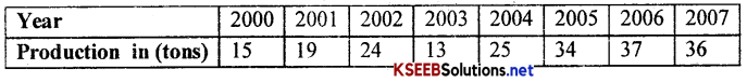
→ If we observe the above table, that the production is increasing, although for some years, it has decreased. The rise or fall of production may be due to some causes or influences or reasons, and are all called ‘factors’.

→ “The factors which are responsible for the fluctuations occurring in the time series are called Components of time series.”

→ The components/variations of time series are classified into four main classes. They are-

1. Secular trend
2. Seasonal trend
3. Cyclical variations
4. Irregular/ Random variations.

Purpose/uses:

The analytical study these factors/ time series will helps to:

• Understand the past, present & future behavior of the data
• Predict / plan for future
• Control present performance and
• Facilitates comparison.

1. Secular trend: ‘The term secular trend/’Trend’ refers to the tendency of the variable to Increase or decrease or to remain steady over a period of time’, e.g. The values of population, prices, sales, literacy etc. are all increasing. As against the death rate, illiteracy, travel by bullock carts is decreasing. The rise or fall may be steep or gradual. But they show increasing trend, if we observe over a sufficiently long period of time.
(Here the time ‘t’ > 1 year)

2. Seasonal trend: The term seasonal variations basically refer to the variations caused annually by the seasons of the year. But also includes the variations of any kind which are periodic in nature and whose period is shorter than one year (Here the time’t'< 1 year). There are two important factors which are responsible for seasonal variations namely
(a) climatic and weather conditions
(b) Customs, habits and traditions of the people.
Ex:

• Sales of cool drinks, ice creams are more in the summer season
• Sale of stationery will be more in June, July.
• The business commercial Bank may reach a peak around the first week of every month.
• Sales of coconuts are always high on Saturday etc.

Hence a clever Businessman will arrange for the production or to maintain stock accordingly to the needs of the season and will earn maximum profit.

3. Cyclical Variations: Cyclical variations are the fluctuations spread over a period of more than one year. (Here time ‘t'< 1 year). Most of the Time series relating to Economics and Business show some kind of cyclical variations. Hence ‘cyclical variation is an oscillatory variation which occurs in four stages, such as:

• Prosperity
• Decline/Recession
• Depression and
• Improvement/Recovery

Business cycle is:

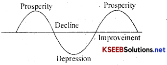
In Prosperity, the curve increases, the business is in boom, the transaction are much more than expected. After reaching the peak of activities the business declines, the curve slopes down. This is called the period of Decline, in Depression the business activities are at the lowest. Then follows a period of improvement in activities and the curve again starts to rise. In this manner the cycle repeats. The interval of time from one prosperity to the other is called the period of cycle. (Here the time ‘t ‘ > OR < 1 year)

4. Irregular or Random variations: Irregular variations are those changes of time series which are irregular in nature and do not show any pattern. The causes of irregular variations are due to accidental happenings such as wars, earth quacks, floods, famine, fire, strikes, etc. These factors are unpredictable. Generally such variations last for a short period.

Methods of measuring of Trend:

Following methods are used for the measurement of trend:

• Graphical method
• Semi-average method
• Moving average methods
• Least squares method

1. Graphical method:
In this method original data will be plotted on the graph. By taking time points on x-axis and the values of the variable on y-axis. The plotted points are joined by a straight line which gives trend. The straight line or the curve will be judgment to the best fit to the data. The graph of a time series is called Historigram.

Merits:

• It is the simplest method.
• It is flexible and adaptable.

Demerits:

• It is affected by personal bias.
• It does not help us to measure exact trend of the time series.
• It is a non-mathematical and so no rigid mathematical formula is laid down for drawing the trend line.

2. Semi-average method:
In this method the given data is divided into two equal parts, with same number of years in two parts and if in case odd number of years by omitting the middle year. The averages are calculated for both the parts. These two averages are called semi-averages. These averages are plotted on a graph, which gives straight line. And this straight line gives us the trend of the time series.

Merits:

• It is simple to understand and easy to calculate.
• It is an objective method of measurement of trend, since everyone who applies this method will get the same trend.

Demerits:

• It is affected by the limitation of arithmetic mean.
• This method cannot used for the measurement of trend.

3. Method of moving averages:
→ In this method simple arithmetic means are calculated successively by taking some specified number of values at a time ( period of moving average ‘m’), say 3, 4, 5 years’. The aim of averaging is to remove the short term variations they are present in the time series of a periodic type. Here the period of moving average (m) is the period covering number of consecutive values taken at a time”.

→ In 3 yearly moving averages, the first moving average is the average of Ist, 2nd and 3 rd observations, and is written against the middle i.e. the 2nd time point. Then dropping the 1st value and adding the next value, 2nd value and continuing this process, until all values are included. Here there are no values for 1 st and last time points

→ If m is even number ie.(m = 2 or 4), first moving averages with period ‘m’ are found, these are not belong to any of the time points and so again ‘moving averages with period 2 of the moving averages are calculated, and are called centered moving averages’. Such calculated values are called trend values (Ŷ)
The graph of a time series is called “Historigram”

Merits:

• This is the simple mathematical method
• If few observations are added to the data the trend values are not affected
• This method is suitable if the time series shows an irregular trend

Demerits:

• Trend values cannot be computed for all years.
• Forecasting/ Future values cannot be determined

4. Method of Least Squares:
In this method a mathematical relation is developed between the time (X) and the values (Y). The relation may be used to fit

• Linear trend
• Quadratic trend
• Exponential

“Method of least square is method of fitting a mathematical relation to the time series such that the sum of squared deviations of the observed and trend values is least”

Principle: Here a relation is derived such that the sum of squares of the deviations of the actual values (Y) and the trend values (Ŷ) is least i.e. Σ(Y – Ŷ)² IS least and Σ(Y- Ŷ) = 0 ; This process results Normal equations, {i.e. In reducing the errors between actual and trend values} ‘The process of minimisation of sum of squared errors result in some equations which are called as normal equations’.

Normal equations are the equations which are used for finding the coefficients (constants say a, b) of the relation which is fitted by the method of least squares.

Merits:

• This method is mathematical, gives accurate trend values
• Trend values can be computed for all time points.
• Future values can be predicted for the given time points.

Demerits:

• This method is tedious
• Difficult to apply the type of Equation.
• Entire calculations has to be done if any observations are added to the time series.

(i) The Straight line/Linear trend equation is: y = a + bx
Normal Equations are
na + bΣx = Σy
aΣx + bΣx² = Σxy
Where, y – actual value,n-number of years x – time, a and b are constants are determined by solving the normal equations. After getting the values of a and b the equation is fitted and the fitted equation is called line of best fit as Ŷ -the trend line.

NOTE: using deviation method always we can get Σx = 0 and so a = \(=\frac{\Sigma y}{n}\) and b = \(\frac{\Sigma x y}{\Sigma x^{2}}\)

(ii) The Quadratic/second degree equation/parabolic trend equation is:
y = a + bx + cx²
Normal Equations are: na + bΣx + cΣx² = Σy;
aΣx + bΣx² + cΣx³ = Σxy
aΣx² + bΣx³ + cΣx⁴ = Σx²y
By solving above three equations using deviation by getting Σx = 0 we get the values of a, b and c and the equation is fitted. And the fitted equation is called curve of best fit as Ŷ -the parabolic trend.

(iii) Exponential trend (Logarithmic trend) is :
y = ab^x ………….. (1)
Where, y denotes time series data, x denotes time, a and b are constants. Taking logarithms on both the sides of (1), we get
log y = log a + x log b ………….. (2)
The values of the constants ‘log a’ and ‘log b’ are obtained by solving the following two normal equations:
n log a + (log b) Σx = Σ log y ………………. (3)
(log a)Σx + (log b)Σx² = Σx log y ……………… (4)
Using deviation by getting Σx = 0 we get the values of ‘log a’ and ‘log b’
From (3), we get n log a = Σ log y; ie., log a = \(\frac{\Sigma \log y}{n}\)
And from (4), we get log b. Σx² = Σx. log y . ie., log b = \(\frac{\Sigma x \log y}{\Sigma x^{2}}\)

2nd PUC Statistics Notes