2nd PUC Statistics Notes Chapter 5 Theoretical Distribution

Karnataka 2nd PUC Statistics Notes Chapter 5 Theoretical Distribution

High Lights of the Topic:

→ The probability distribution of a random variable obtained on the basis of some theoretical assumptions are known as theoretical or probability distributions.

→ Discrete probability distributions: Probability distribution of a discrete random variable is known as discrete probability distribution.

Ex: Number of Heads obtained when three coins are tossed, Number of female children in a family, Number of accidents occurring in a city in a day, drawing balls without replacement from a bag of different coloured balls etc. are discrete variable examples. The following probability distributions are used to deal such examples.

• Bernoulli distribution
• Binomial distribution
• Poisson distribution
• Hyper-geometric distribution

Continuous Probability Distributions:
Probability distribution of a continuous random Variable is known as continuous probability distribution.

Ex: Height/ Weight/ Marks obtained by a of class of students, Age/Wages/Income of employees of a factory etc. are all continuous variable examples. The following probability distributions are used to deal with such examples.

• Normal distribution
• Chi-square distribution
• Student’s t-distribution

Discrete Probability Distributions:

Bernoulli Distribution:

{Introduced both Bernoulli and Binomial distributions by Mr.James Bernoulli} A random experiment which has only two outcomes as ‘success’ and ‘failure’ where
P(succeess) = p & P(failure) = q or (1 – p) is called Bernoulli Trail or Experiment.

Examples:
1. Tossing a fair coin once, and getting out comes as Head (success-p) or Tail (failure-q)

2. A new born baby may be male (p) or female (q)

3. A bomb is dropped on a target may hit (p) or may not hit (q)

4. An item chosen at random may be defective or not

5. Rolling a die and getting no. 6 (success) or not (other numbers). The probability mass function (p.m.f) is:
P(x) = P^x (1 – P)^{1 – X};                             where p > 0, and X = 0, 1
OR P(x) = P^x q^{1 – x} x = 0, 1                   Where p is probability of success (0 < p < 1)

→ Here x-is discrete and is called Bernoulli variate.

• The Bernoulli distribution with the parameter p denoted by B(p)
• The distribution can also be written as:

→ A random variable x assumes values 1 and 0 with respective probabilities p and (1 – p) is called Bernoulli variate
The Bernoulli distribution can also be writtens is:

Where p-the probability of success

Properties/Features:

• Here p-is the parameter, is a constant
• Mean = E(x) = p,
• var(x) = p (1 – p) or pq
• For the distribution Mean(p) > Variance
  s.d(x) = \(\sqrt{p(1-p)}\) or \(\sqrt{p q}\)

Binomial Distribution:

Bernoulli distribution tends to Binomial distribution:
If x₁, x₂, x₃ …………. x_n are independently identically distributed (i.i.d.) Bernoulli variates, then (x₁ + x₂ + x₃ + ………… + x_n) is a Binomial variate with parameters n and p

Conditions/Assumptions that Binomial distribution can be applied:

• Trails are repeated number of times and are independent.
• Each trail is a Bernoulli trial with two outcomes as success and failure
• The probability of success ‘p’ should be constant for each of the trails
• Experiment should be conducted under similar conditions for a fixed number of trails say ‘n’.

Examples:

• Number of heads obtained when 5 coins are tossed
• Number of male children in a family of 3 children
• Number-of defective articles in a random sample of 7 articles
• Number of bombs hitting a target when 4 bombs are dropped on it.

Similarly number of accidents, deaths, infections, contracting a disease, literates, mango trees among the trees etc.
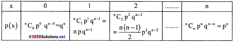
The p.m.f is: P(x) = nc_xP^xq^{n – x}; Where x = 0, 1, 2, 3 …………….. n, and range of p: 0 < P < 1
Here x is discrete and is called Binomial variate.

Properties / Features:-
→ n & p are the parameters

→ Range: 0, 1, 2, n

→ The Binomial distribution with the parameters n, p denoted by B(n, p)

→ Mean = np, var(x) = npq, sd(x) = √var(x) = \(\sqrt{\mathrm{npq}}\)

→ Relation between mean and variance: mean > variance, ie. np > npq

→ Binomial distribution is symmetric when p = \(\frac{1}{2}\) (i.e., β₁ = 0 non-skewed).

→ Expected /Theoretical frequency = T_x = p(x).N

→ The distribution is called symmetric when p = q

→ Recurrence relation to get theoretical frequency = T_x = \(\frac{n+1-x}{x} \frac{p}{q} T_{x-1}\)

→ Recurrence relation to get theoretical P(x) = \(\frac{n+1-x}{x} \cdot \frac{p}{q} p_{x-1}\)

→ The terms of B.D are:

→ If p > \(\frac{1}{2}\) or q >\(\frac{1}{2}\) then binomial distribution is positively skewed (i.e., β₁ > 0).

→ If P < \(\frac{1}{2}\) or q < \(\frac{1}{2}\), then binomial distribution is negatively skewed (i.e., β₁ < 0).

Poisson Distribution

{French mathematician S.D.Poisson ini 837 used to describe the behavior of rare happening of events.}

Examples:

• Number of telephone calls received in one minute
• No. of printing mistakes in a book/typing mistakes (typographical errors) in a page.
• No. of accidents/deaths occurring in a city in a day
• No. of defective articles manufactured in a lot by a firm.
• Number of vehicles crossing a junction in one minute.

Binomial distribution tends to Poisson distribution under the following conditions:
(i) When n is large ie., n → ∞
(ii) When P is very small ie., p → 0 and
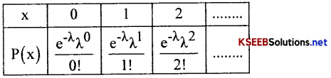
(iii) Mean = np = λ is fixed / constant, which is parameter of the Poisson distribution Poisson distribution is:
A distribution which has the following p.m.f. as:-
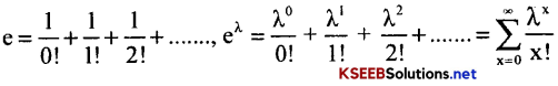
P(x) = \(\frac{e^{-\lambda} \lambda^{x}}{x !}\); where x = 0, 1, 2, ………….. ∞ and m > 0, (λ read lamda)
Here x is discrete is called Poisson variate.

Properties Features:

• e-Euler’s constant (2.7184) is the base of the natural number,
• Range : 0, 1, 2 …………… ∞.
• λ – Parameter
• Mean = E(x) = λ, Var(x) = λ,
• Here mean = variance; is the relation b/w mean and variance
• Theoretical frequency/Expected frequency = T_x = P(x).N
• Recurrence relation to get theoretical frequencies T_x = \(\frac{\lambda}{x} \mathrm{~T}_{\mathrm{x}-1}\)
• First three Terms of distribution:-

Note:

Hyper-geometric distribution:

Examples:-

• Number of girls in student representatives when 6 students are selected from 50 boys and 30 girls of a class.
• Number of coffee drinkers in a sample of 5 selected from a teaching staff of 15 coffee drinkers and 12 tea drinkers.
• Number of red balls drawn in a draw of 3 balls urn with 5 red and 4 black balls.
• Number of computer illiterates in a selection of 5 persons from an office of 10 men and 8 women.

A probability distribution which has the following probability mass function (p.m.f) as;
P(x) = \(\frac{{ }^{a} C_{x}{ }^{b} C_{n-x}}{{ }^{a+b} C_{n}}\); where x = 0, 1, 2, ………….. min(a, n); Where a, b and n are positive integers (> 0) Here X is discrete called Hypergeometric variate.
Note: Here n ≤ (a + b) .

Properties/Features:

1. a, b and n are the parameters.

2. Range: 0, 1, 2, ……….. min (a, n).

3. For a hyper-geometric distribution mean = \(\frac{\mathrm{na}}{\mathrm{a}+\mathrm{b}}\)

4 Var(x) = \(\frac{n a b(a+b-n)}{(a+b)^{2}(a+b-1)}\) and S.D = √var(x)

5. Hypergeometric distribution tends to Binomial distribution when:
(i) a is large ie. a → ∞
(ii) b is large ie. b → ∞ and
{Binomial distribution is a limiting form of Hyper-geometric distribution with parameters n and p = \(\frac{a}{a+b}\)}.

6. A hyper-geometric distribution with parameters a, b and n is denoted by H(x; a, b, n) or H(a, b, n).

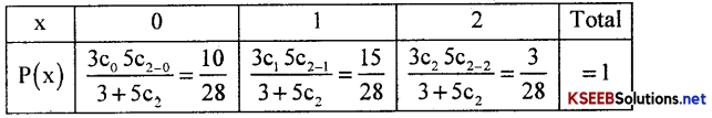
7. If a = 3 , b = 5 and n = 2 the Hypergeometric distribution can be written as:
The terms:

Continuous Probability Distributions

Normal Distribution

[Introduced and developed by De-Moivre, Pierre Laplace, Carl F-Gauss, also this distribution is called Gaussian distribution]

→ The Normal distribution is a limiting case of the Binomial distribution ie. Binomial tends to Normal, under following conditions:

• The number trails ‘n’ becomes very large, ie. n → ∞
• Neither p nor q is very small, and np = µ, σ = \(\sqrt{\mathrm{npq}}\)

→ In Poisson distribution with parameter λ becomes large we use normal distribution as an approximation ie. Poisson tends to Normal when, λ → ∞ and mean = µ = λ, σ = √λ

Examples:

• Ht. / Wt. of students of a class
• Wt. of apples grown in an orchard
• I.Q. of a large group of children.
• Marks scored by students in an examination.
• Wages / Income of employees.

A probability distribution which has the following probability density function (p.d.f.) as:-

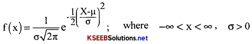
Here x is continuous and is called Normal variate.

For a N.D:

• Range: (- ∞, ∞)
• p and a are parameters,
• In the distribution π = 3.14, e = 2.718 euler’s constant .
• Mean = E(x) = µ Var(x) = σ², S.D = σ
• A normal variate with parameters and is denoted by N(µ, σ²)

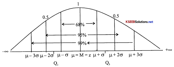
Properties of Normal distribution /Normal curve: –

A Normal distribution with parameters is and a has the following properties:
1. The curve is bell shaped:

• The curve is symmetrical (non-skew) β₁ = 0
• Mean = Median = Mode, ie. Mean, Median and Mode are all equal.

2. The Quartiles Q₁ & Q₃ are equidistant from the Median are given by:
Q₁ = µ – 0.6745σ and Q₃ = µ + 0.6745µ (Here, Q₂/Z/µ = \(\frac{\mathrm{Q}_{1}+\mathrm{Q}_{3}}{2}\))

3. The curve is Asymptotic to the x-axis ie., the curve touches the x-axis at -∞ & + ∞.

4. The curve has Points of Inflexion at µ ± σ.

5. For the distribution: S.D = σ, Q.D = \(\frac{2}{3}\)σ, M.D = \(\frac{4}{5}\)σ, Here QD = \(\frac{\mathrm{Q}_{3}-\mathrm{Q}_{1}}{2}\)

6. The distribution is mesokurtic β₂ = 3.

7. The total area under the curve is one (1):
ie. (a) P(µ – σ < X <µ + σ) = 0.6826,
(b) P(µ – 2σ < X < µ + 2σ) = 0.9544,
(c) P(µ – 3σ < X > µ + 3σ) = 0.9974

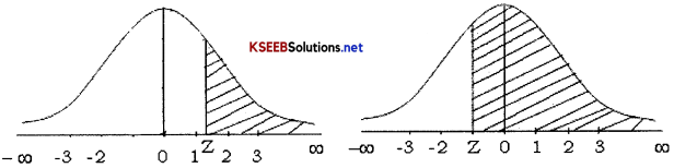
Standard Normal Variate (SNV): A Normal variate with mean µ = 0 and S.D. σ = 1 is called
S.N.V. Denoted by Z ; ie, Z = \(\frac{x-\mu}{\sigma}\) ~ N(0, 1).

The P.d.f of SNV is – f(z) = \(\frac{1}{\sqrt{2 \pi}} \mathrm{e}^{-\frac{Z^{2}}{2}}\); where – ∞ < Z < + ∞, Here Z = \(\frac{x-\mu}{\sigma}\);

Let x be a normal variate with, mean µ and S.D (σ), then Z is Standard Normal Variate. To find any probability regarding X, S.N.V is used to find the probability under the area under the Normal curve from 0 to z or from z to ∞

Chi-Square Distribution

Note:

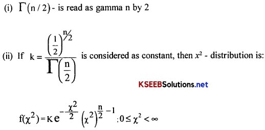
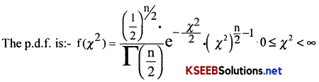
Definition of x distribution:- Let Z₁, Z₂, Z₃ …… Z_n are n S.N.V’s ; then
x² = Z₁² + Z₂² + Z₃² + + Z_n² ~ x²(n)

Features/Properties:

• Parameter = n;
• Range (0, ∞)
• Mean = n, *Variance = 2n, * SD. = √var9(x) = \(\sqrt{2 n}\)
• Mode = (n – 2) for n > 2,
• The curve is positively skewed for n > 2 (β₁ > 0).
• χ² – distribution is leptokurtic (β₂ > 3).
• Total area under the χ² – curve is equal to 1.
• χ² – distribution tends to follow standard normal distribution When n is large ie. n → ∞
• χ² – distribution is leptokurtic (β₂ > 3).

Application:

• Test for population variance
• Test for Goodness of Fit
• Test for Independence of Attributes.

Students’s T-Distribution

This distribution developed by W.S.Gossett in 1908.it is derived from the normal distribution.

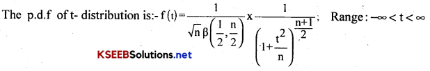
Note 1: The t-distribution can also can be written:
If k = \(\frac{1}{\sqrt{n} \beta\left(\frac{1}{2}, \frac{n}{2}\right)}\)

Then; f(t) = k × \(\frac{1}{\left(1+\frac{t^{2}}{n}\right)^{\frac{n+1}{2}}}\) Range; – ∞ < t < ∞

Note 2: t – variate with n d.f. is denoted by t(n).

Features / Properties:

• parameter ‘n’ called degrees of freedom;
• Range: (-∞, ∞)
• The t-curve is bell shaped
• Mean = 0,(X̄ = M = Z = 0),
• Var(x) = \(\frac{\mathrm{n}}{\mathrm{n}-2}\) for n > 2; and S.D(x) = \(\sqrt{V(x)}\)
• The t-distribution is symmetrical about t = 0 ie. β₁ = 0.
• The distribution is leptokurtic β₁ > 3.
• t-distribution is asymptotic to X-axis.
• t-distribution tends to Normal distribution when n is large.

Application:- t – distribution is used in small sample tests of testing hypothesis :

• To test for mean,
• Test for equality of means,
• Test for equality of population means when observations are paired (paired t-test).

2nd PUC Statistics Notes