Karnataka 2nd PUC Statistics Notes Chapter 6 Statistical Inference
High Lights of the Topic:
Parameter:
→ A statistical constant of the population is called a parameter.
→ Statistical constants of the population such as Mean (x̄), S.D (σ) & Proportion-P0 Or P are Parameters
Parameter space:
→ The set of all the admissible values of the population parameter is called parameter space. Suppose X ~ N(µ, σ2), then parameter space for µ = {- ∞ < µ < ∞} and for a = σ = {0 < σ < ∞}
![]()
Statistic:
→ A function of the sample values is called a statistic.
→ Statistical measures computed from the samples such as Mean (x), S .D (s), & proportion- p are statistic.
Sample space:
→ The set of all samples of size W that can be drawn from population is called sample space.
Sampling distribution:
→ The distribution of the values a statistic for different samples of same size is called its sampling distribution.
→ Many sample means (x) can be tabulated in the form of frequency distribution from the population, the resulting distribution is called sampling distribution of sample mean (X̄). Similarly sampling distribution of sample S.D (s), sampling distribution of sample proportion (p) etc.
Standard Error:
→ The standard deviation of the sampling distribution of sample statistic is called standard error (S.E) of statistic
S.E (X̄) of sample mean:
Consider a population whose mean ‘μ’ and S.D. ‘σ’. Let a random sample of size ‘n’ be drawn from this population. Then the sampling distribution of X̄ has mean ‘μ’ and Standard deviation:
SE(X̄) = \(\frac{\sigma}{\sqrt{n}}\)
If ‘σ’ is not available use’s’, SE(X̄) = \(\frac{\mathrm{s}}{\sqrt{\mathrm{n}}}\) =; s-sample S.D
![]()
S.E of difference of means/ S.E(x̄1 – x̄2):
→ Let a random sample of size ‘nl’ be drawn from a population whose mean is µ1, and s.d. σ1. Also, let a random sample of size ‘n2‘ drawn from another population whose mean is µ2, and s.d. σ2. Let x̄1 and x̄2 are the means 1st and 2nd samples drawn from the populations,
→ Then difference of sample means (x̄1 – x̄2) has mean ‘(µ1 – µ2)’ and
S.E. (x̄1 – x̄2) = \(\sqrt{\frac{\sigma_{1}^{2}}{n_{1}}+\frac{\sigma_{2}^{2}}{n_{2}}}\) OR S.E. (x̄1 – x̄2) = \(\sqrt{\frac{s_{1}^{2}}{n_{1}}+\frac{s_{2}^{2}}{n_{2}}}\); Where s1 and s2 are sample standard deviations
S.E of sample proportion/ S.E (p1 – p2):
→ In a population let PQ be the proportion of units which posses the attribute. From such a population suppose a random sample of size ‘n’ is drawn.
→ Let ‘x’ of these units belongs to the class ‘posses the attribute’ then p = \(\frac{x}{n}\), is the sample proportion of the attribute. Then ‘p’ has mean ‘P0’ and S.E(p) = \(\sqrt{\frac{\mathrm{P}_{0} \mathrm{Q}_{0}}{\mathrm{n}}}\); Q0 = 1 – P0
→ Here, in order to avoid confusion between population proportion (P) and sample proportion (p): ‘caps’ P is used as P0 and Q as Q0
S.E. of difference of the sample proportions/S.E (p1 – p2):
→ Let a random sample of size ‘n1‘ be drawn from a population with proportion ‘P01‘ of an attribute. Let x1 units in the sample posses the attribute. Then the sample proportion of 1 st sample: P1 = \(\frac{x_{1}}{n_{1}}\).
→ Similarly n2 → P02; x2 → p2 = \(\frac{\mathrm{x}_{2}}{\mathrm{n}_{2}}\).
→ Hence the difference of (p1 – p2) has mean (P01 – P02) and S.E(p1 – p2) = \(\sqrt{\frac{\mathrm{P}_{01} \mathrm{Q}_{01}}{\mathrm{n}_{1}}+\frac{\mathrm{P}_{02} \mathrm{Q}_{02}}{\mathrm{n}_{2}}}\)
→ If P01 = P02 = P0, ie, two population proportions are same, the
S.E (p1 – p2) = \(\sqrt{\mathrm{P}_{0} \mathrm{Q}_{0}\left(\frac{1}{\mathrm{n}_{1}}+\frac{1}{\mathrm{n}_{2}}\right)}\)
Uses (utility) of S.E’s :
- It is used in theory of estimation, to decide the efficiency and consistency of the statistic as an estimator.
- It is used in interval estimation, to write down the confidence intervals.
- It is used in testing of hypothesis, to test whether the difference between the sample statistic and the population parameter is significant or not, ie. to standardize the distribution of test statistic.
Theory of Estimation:
→ The statistic used for the purpose of estimation of unknown population parameter is called an Estimator. Whereas Estimate is a numerical value of the computed from a given set of sample values.
→ Suppose if a sample statistics (x̄) is used to find out the value of the population parameter (µ), such a value is called the Estimator of the parameter. And the value of the Estimator is called the Estimate.
→ Thus, the statistic x̄ is an Estimator of µ and its value x̄ is the Estimate.
→ Similarly ‘s’ (sample s.d) is an Estimator of ‘σ’ (population s.d) and its value ‘s’ is the Estimate.
→ When estimating parameters of the populations, the following two types of estimates are possible.
- Point Estimation
- Interval Estimation.
![]()
1. Point Estimation:
In Point Estimation a single statistic used to provide an estimate of the population Parameter. “While estimating unknown parameter, if a single value is proposed as an estimate is called point estimation”
{i.e., the estimate of a population parameter given by a single number is called point estimation.} for example the mean pass number of 50 students will be 55.
2. Interval Estimation:
→ If an interval is proposed as an estimate of the unknown parameter, then it is interval estimation.
In Interval Estimation:
- “While estimating an unknown parameter, instead of a specific value, an interval is proposed, which is likely containing the parameter is called Interval estimation”
- A confidence interval is an interval within which the unknown population parameter is expected to lie. (The interval which is likely to contain the parameter)
- The probability that the confidence interval contains the parameter is called confidence coefficient.
- The Intervals within which the most probable value of parameter contains are called confidence limits. Ie the limits T1 and T2 of the confidence interval are called confidence limits.
Testing of Hypothesis
Statistical Hypothesis:
A statistical Hypothesis is a statement regarding the statistical distribution of the population OR It is a statement/assertion made regarding the parameters of the population denoted by H.
Ex:- H: The population has mean = p (= 25)
H: The population is Normally distributed with mean µ = 25, and s.d. σ = 2
Null Hypothesis:
“Null Hypothesis is a hypothesis which is being tested for possible rejection under the assumption that it is true. Denoted by H0”
Ex: H0: The population mean is µ (= 25) OR {H: µ = µ0}
H0: The means of the two populations are equal OR {H0: µ1 = µ2}
Alternative Hypothesis:
“The hypothesis which is being accepted when the null hypothesis is rejected is called alternative hypothesis. Denoted by H1”
Ex: H1: The population mean differs from (H1: µ ≠ µ0 (25))
Also H1 may be H1: µ < µ0(25) or H1: µ > µ0(25)
H1: The means of the two populations are not equal, may be less than or more than
{H1: µ1 ≠ µ2 or H: µ < µ2 or H1 = µ1 > µ2}
![]()
Simple Hypothesis:
“A hypothesis which completely specifies the parameter of the distribution is called simple hypothesis”.
Ex: H: < µ0 (25) is a simple hypothesis
H: The population is Normally distributed with mean µ = 25 and σ = 2
Composite Hypothesis:
“A hypothesis which does not completely specify the parameter of the distribution is a composite hypothesis”
Ex: H: The population is normally distributed with mean µ > 25
Test statistic:
→ “Test statistic is the statistic based on whose distribution testing is conducted”
→ Suppose for testing H0 = µ = µ0, the test statistic is Z = \(\frac{\overline{\mathrm{x}}-\mu}{\mathrm{S} . \mathrm{E}(\overline{\mathrm{x}})}\) i.e., Z = \(\frac{\overline{\mathrm{x}}-\mu}{\sigma / \sqrt{\mathrm{n}}}\) OR Z = \(\frac{\overline{\mathrm{x}}-\mu}{\mathrm{s} / \sqrt{\mathrm{n}}}\)
→ Here “the statistical distribution of the test statistic under which the Null Hypothesis stated is called Null Distribution”
Critical Region:
→ “The set of all those values of the test statistic which lead to the rejection of the null hypothesis is called critical region (to), also called as Rejection region”.
→ “The set of those values of test statistics which lead to the acceptance of the null hypothesis is called acceptance region(s – ω)”.
Critical value:
→ “The value of test statistic which separates the critical region (i.e. rejection region) and acceptance regions is called the critical value or significance value”.
→ Usually denoted by ± K/-K1, K2. Its value depends of level of significance (α) used ie, either at 5% (0.05) or 1% (0.01).
Here for α = 5% ± K1 = ± 1.96 and ± k2 = ± 2.58 for two tail test
for α =1 % ± K1 = ± 1.65 and ± k2 = ± 2.33 for one tail test
![]()
When a statistical hypothesis is tested there are four possible decisions are made as below:
- If the Null hypothesis is true and our test accepts it -Correct decision
- If the Null hypothesis is true but our test rejects it -Type I Error
- If the Null hypothesis is false and our test accepts it -Correct decision
- If the Null hypothesis is false but our test accepts it – Type II Error
Type I:-
“Type I Error is taking a wrong decision to reject the null hypothesis when it is actually true” ie. (Rejecting H0 when it is true)
Type II Errors:-
“Type II Error is taking a wrong decision to accept the null hypothesis when it is actually not true” (Accepting H0 when it is not true)
Level of Significance (α):
“It is the probability of rejecting the null hypothesis when it is actually true denoted by α”.
i. e., α = P (Type I Error) OR ‘prob. of occurrence of Type I error is called Level or significance’, which is referred as ‘producers risk’. Usually is fixed at 0.05 or 0.01.
Here α = P (Type I Error) is also called as Size of the test.
Power of a Test:
“It is the probability of rejecting the null hypothesis when it is not true, denoted by (1 – β)”. ie., Here β = P(Type II Error) which is referred as ‘consumers risk’
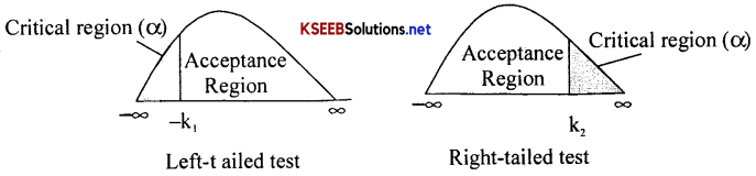
One-Tailed and Two-Tailed Test:
→ While testing of null hypothesis, a two-tailed test of hypothesis will reject the H0 if the sample statistic is significantly higher than or lower than the parameter.
→ Thus in two-tailed test the rejection region is located in both the tails.
→ Whereas is one tailed test rejection region is located in one side ie. Right or left tailed.
Definition:
→ “If the critical region is considered at one tail of the null distribution of the test statistic, the test is one-tailed test”
Ex:- When Ho: µ = µ0 versus H1: > µ0, then it is a right tailed test;
When Ho: µ = µ0 versus H1: < µ0, then it is a left tailed test.
Definition:
“If the critical region is considered at the both the tails of the null distribution of the test statistic, the test is two-tailed”
Ex:- When H0: µ = µ0 versus H1: µ ≠ µ0, then it is two tailed test.
When H0: µ1 = µ0 versus H1: µ1 ≠ µ0, then it is two tailed test.
![]()
Test Procedure:
Following are steps involved in any test of hypothesis:
- Setting up null and alternative hypothesis, ie., H0 & H1
- Identifying the test statistics and its distribution as, Z, χ2, t, etc.,
- Selecting level of significance (α) and finding the critical value.
- Making decision and conclusion.